
Jupyter notebooks make it possible to produce interactive simulations/animations that are controlled by interactive widgets, such as sliders and buttons. When appropriately configured, changing the value of a slider or clicking a button triggers Python to run an update function, which can then ask the notebook frontend to redisplay something. The details are a bit tricky, but the result is great and work the effort to debug.
I will assume that the simulation is running in Jupyter Lab, that ipympl and ipywidgets have been installed, so that matplotlib output is displayed in an interactive widget. That is, you are successfully able to use %matplotlib widget in the notebook.
We model a damped simple harmonic oscillator being driven sinusoidally. Rather than handling the dynamic situation, we will show the amplitude and phase of the oscillator’s motion as a function of the drive frequency. The equation of motion is \begin{equation} m\ddot{x} = -b \dot{x} - m\omega_0^2 x + F_{\rm drive} \end{equation} Divide through by \(m\) and define \(\beta = b/2m\) to get \begin{equation} \ddot{x} + 2 \beta \dot{x} + \omega_0^2 x = \frac{F_{\rm drive}}{m} \end{equation} I will assume that the drive force is the real part of \(F_0 e^{-i\omega t}\) and look for a steady-state solution of the form \(x = A e^{-i\omega t}\). Substituting these into the differential equation, we get \begin{equation} (-\omega^2 - 2 \beta \omega i + \omega_0^2) A e^{-i \omega t} = \frac{F_0}{m} e^{-i \omega t} \end{equation} Therefore, \begin{equation} A = \frac{F_0/m}{(\omega_0^2 - \omega^2) - 2 \beta \omega i} \end{equation} I now want to express the denominator in polar form, so define \(\Delta = \sqrt{(\omega_0^2-\omega^2)^2 + 4 \beta^2 \omega^2}\) and \(\tan \varphi = \frac{2 \beta \omega}{\omega_0^2 - \omega^2}\). Then \begin{equation} A = \frac{F_0/m}{\Delta} e^{i\varphi} \end{equation}
I have implemented the simulation in a class DDSHO, with commented methods shown below. The computational part is straightforward and follows the algebra shown above. The
trickier part has to do with the controls and the updates.
plot method is first called, a figure and axes are created and their default properties are defined.widgets.FloatSliders, and set to have continuous updates.widgets.interact is called to get the method change called whenever there is a change in the state of any of the sliders.change method reads the value of every slider, updates the physical parameters in the DDSHO object, and recomputes the graphs by calling update.class DDSHO:
"""
Simulate a damped simple harmonic oscillator driven steadily at frequency
ω. Plot the amplitude and phase of the motion with respect to the drive as
a function of frequency.
"""
def __init__(self, **kwargs):
"""
We will provide explicit default values for the physical parameters and
allow the user to override them using keyword arguments. The overrides
will be made in `self.set_properties` so that future overrides generated
by the sliders can be handled in the same way.
"""
self.m = 1
self.b = 0.2
self.k = 1
self.F = 1
self.fig = None
self.ax = None
self.set_properties(**kwargs)
def set_properties(self, **kwargs):
"Update the physical parameters of the simulation"
okay = ['m', 'b', 'k', 'F']
for k, v in kwargs.items():
if k in okay:
setattr(self, k, v)
else:
print(f"Unknown property {k} passed to set_properties")
self.ω0 = np.sqrt(self.k / self.m)
self.β = self.b / (2 * self.m)
def __call__(self, ω):
"Return the amplitude and phase for (each value in) ω"
dω = self.ω0**2 - ω**2
ϕ = np.degrees( np.atan2(2 * self.β * ω, dω) )
a = self.F / self.m / np.sqrt(dω**2 + (2 * self.β * ω)**2)
return a, ϕ
def update(self):
"Update the graphs"
l = self.lines
a, ϕ = self(self.ω * self.ω0)
amax = 10**np.ceil(np.log10(np.max(a)))
amin = 10**np.floor(np.log10(np.min(a)))
l['a'].set_data(self.ω, a)
l['ϕ'].set_data(self.ω, ϕ)
self.axs[0].set_ylim(amin, amax)
title = self.axs[0].set_title(self.title())
return (*list(l.values()), title)
def title(self):
fmt = r"$\beta = %.3g$, $F_0/m = %.3g$"
return fmt % (self.β, self.F / self.m)
def plot(self, npts=201, **kwargs):
if self.fig is None:
# Create the plot (we just do this once)
self.fig, self.axs = plt.subplots(nrows=2, sharex=True, figsize=kwargs.get('figsize'))
for ax in self.axs:
ax.set_xscale('log') # for Bode plots
ax.grid()
self.axs[0].set_yscale('log') # top one will be the amplitude
self.axs[0].set_ylabel('$|A|$')
self.axs[1].set_ylabel(r'$\varphi$ (°)')
self.axs[1].set_xlabel(r'$\nu/\nu_0$')
# We will show a decade on either side of the natural frequency
self.ω = np.logspace(-1, 1, npts)
a, ϕ = self(self.ω) # evaluate the amplitude and phase
self.lines = dict()
l1, = self.axs[0].plot(self.ω, a, c='#AA0000', lw=2, label="$|A|$")
self.lines['a'] = l1
l2, = self.axs[1].plot(self.ω, ϕ, c='#00AA00', lw=2, label=r"$\varphi$")
self.lines['ϕ'] = l2
# Now provide a descriptive title
self.axs[0].set_title(self.title())
# Create widgets for k, b, m, F
# keep track of them in a dictionary
self.widgets = dict()
# Create widgets for k, b, Ω, N
self.widgets = dict()
for c in ('k', 'b', 'm', 'F'):
self.widgets[c] = widgets.FloatSlider(
value=getattr(self, c),
min=0.02, max=10, step=0.02,
description=f"{c}: ", continuous_update=True,
readout_format='.2f')
# Activate the widgets so self.change gets called when they are updated
widgets.interact(self.change, **self.widgets)
def change(self, **kwargs):
"""
Update the physical parameters using the current values of the sliders
and remake the graphs.
"""
self.set_properties(**kwargs)
self.update()
The result of a call to
d1 = DDSHO()
d1.plot()
is shown in Fig. 1. As the user alters any of the slider values, the plots update continuously.
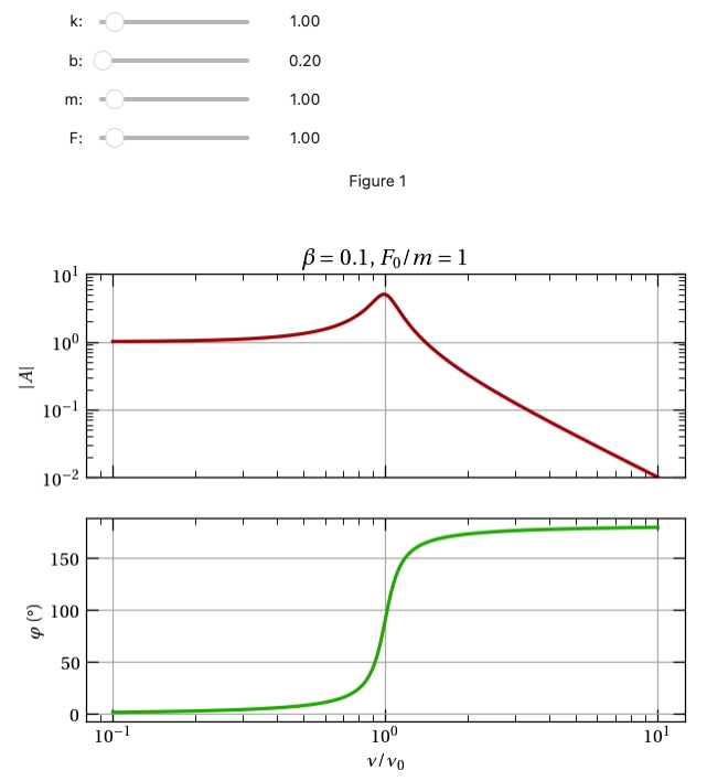
Figure 1 — The Bode plot (and phase plot) of a damped, sinusoidally driven SHO.