
There are many situations in which we wish to use random numbers to solve problems, either because the underlying physical processes have an element of randomness or because the parameter space is too large to sample exhaustively. The starting point for a variety of random distributions is the uniform deviate, such as a random integer between 0 and some maximum value \(N\).
Starting in 1949, a particularly simple sort of “random” number generator was used to approximate truly random numbers. It is called a linear congruential generator (LCG) and has the simple form \begin{equation}\label{eq:LCG} I_{j+1} = (a I_j + c) \; \mathrm{mod} \; m \end{equation} with carefully chosen multiplier \(a\), constant \(c\), and modulus \(m\) to make the period equal to the modulus. If the constant \(c\) is zero, it is called a multiplicative linear congruential generator (MLCG). Both approaches are obsolete; do not use them! They tend to produce values that lie on distinct hyperplanes in multidimensional space. We’ll illustrate a problem using a MLCG in the next section.
A workhorse random number generator must pass a battery of tests of randomness. Examples include:
There are plenty of others, as mentioned in Numerical Recipes, which references the “Diehard” battery of statistical tests with the caveat to be sure that said Diehard includes the so-called “Gorilla Test.” How’s that for colorful?!
As an illustration of the Period test run on a lousy generator (a naive LCG), we can use the following Python code to construct such a generator:
class LCG:
    def __init__(self, a, c, m, x0=3829483):
        self.x = x0
        self.a = a
        self.c = c
        self.m = m

    def __call__(self):
        self.x = (self.a * self.x + self.c) % self.m
        return self.x / self.m

    @property
    def zero_mean(self):
        return 2 * self() - 1

def chisqtest(udev, nbins: int=100):
    """
    Given an array of uniform deviates on [0,1), compute χ^2 and return
    the probability to exceed.
    """
    from scipy.stats import chi2
    expected = len(udev) / nbins
    h, edges = np.histogram(udev, bins=nbins, range=(0,1))
    chisq = np.sum((h - expected)**2) / expected
    return chisq, float(1 - chi2.cdf(chisq, df=nbins-1))

# Testing/plotting routine
def test_rng(gen, name: str, N: int=10000, figsize=(10,5)):
    v = gen.uniform(size=N)
    ch, Pexceed = chisqtest(v)
    mn = v.mean()
    fig, axs = plt.subplots(ncols=2, figsize=figsize)
    axs[0].plot(np.cumsum(gen.zero_mean(N)), c=fs.traces[0], lw=0.5)
    axs[1].hist(v, bins=100, color=fs.traces[1], alpha=0.25)
    axs[0].set_title(f"Mean = {mn:.4f}")
    axs[0].set_ylabel("Cumulative Sum")
    axs[1].set_title(r"$\chi^2 = %.2f$, PTE $= %.2f$" % (ch, Pexceed))
    return fig

# Now create a poorly designed MLCG and test it
poor = LCG(899, 0, 32768)
test_rng(poor, "LCG")
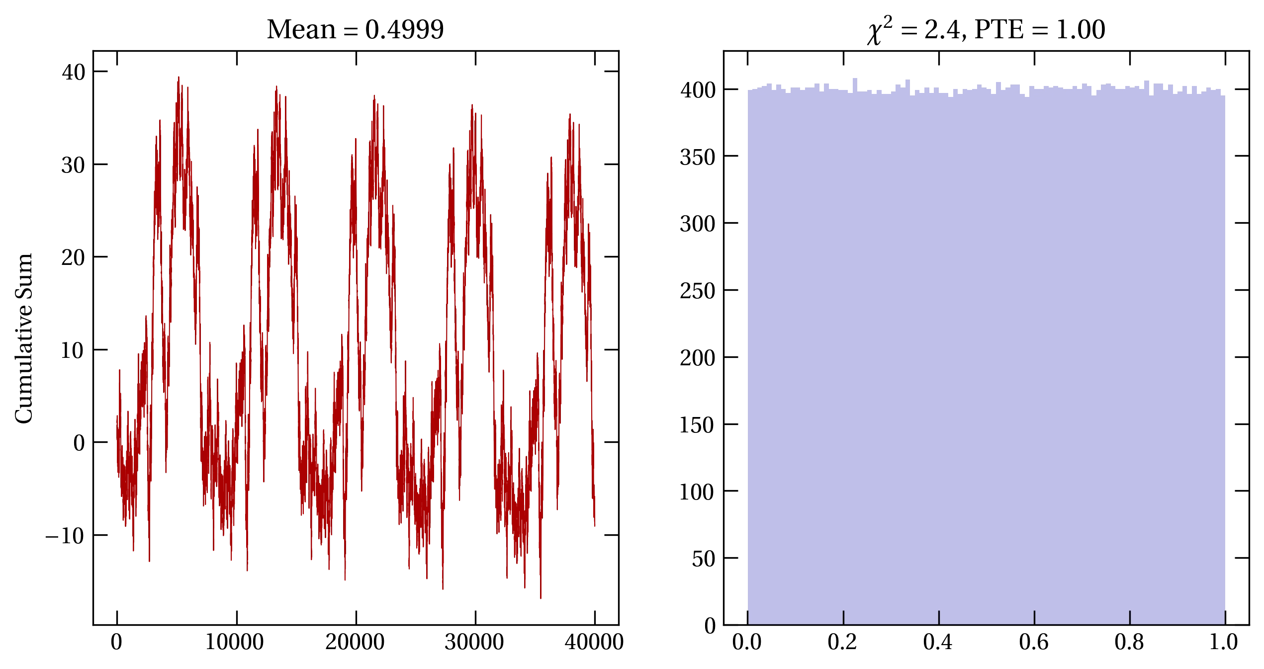
Figure 1 — (left) Period test of a poorly designed MLCG with \(a=899\), \(c=0\), and \(m=32768\), revealing a troublingly short period. (right) Histogram of the same generator, the associated value of \(\chi^2\), and the probability to exceed (PTE) this value of \(\chi^2\). Clearly, the histogram is too even.
A generator based on the xor operation and bit shifting is generally efficient and produces values that pass a number of tests for randomness. Recall that the exclusive or of two bits is 0 if the bits are the same and 1 if they are different. A simple 64-bit xorshift algorithm involves three steps:
import numpy as np

class MyRNG:
    def __init__(self, seed=184738293):
        assert isinstance(seed, int) and seed != 0
        self._x = np.array([seed], dtype=np.uint64)

    def int(self):
        self._x = self._x ^ (self._x >> 21)
        self._x = self._x ^ (self._x << 35)
        self._x = self._x ^ (self._x >> 4)
        return self._x

    @property
    def zero_mean(self):
        n = self.int()
        v = (n & 0x00FFFFFF) / 0x01000000
        return 2 * v - 1
The set of three integers (21, 35, 4) make a good xorshift random number generator. Other sets of three shift integers are certainly possible, as discussed in Numerical Recipes.
mrng = MyRNG()
better = [mrng.zero for n in range(1000000)]
fig, ax = plt.subplots()
ax.plot(np.cumsum(better), lw=0.5)
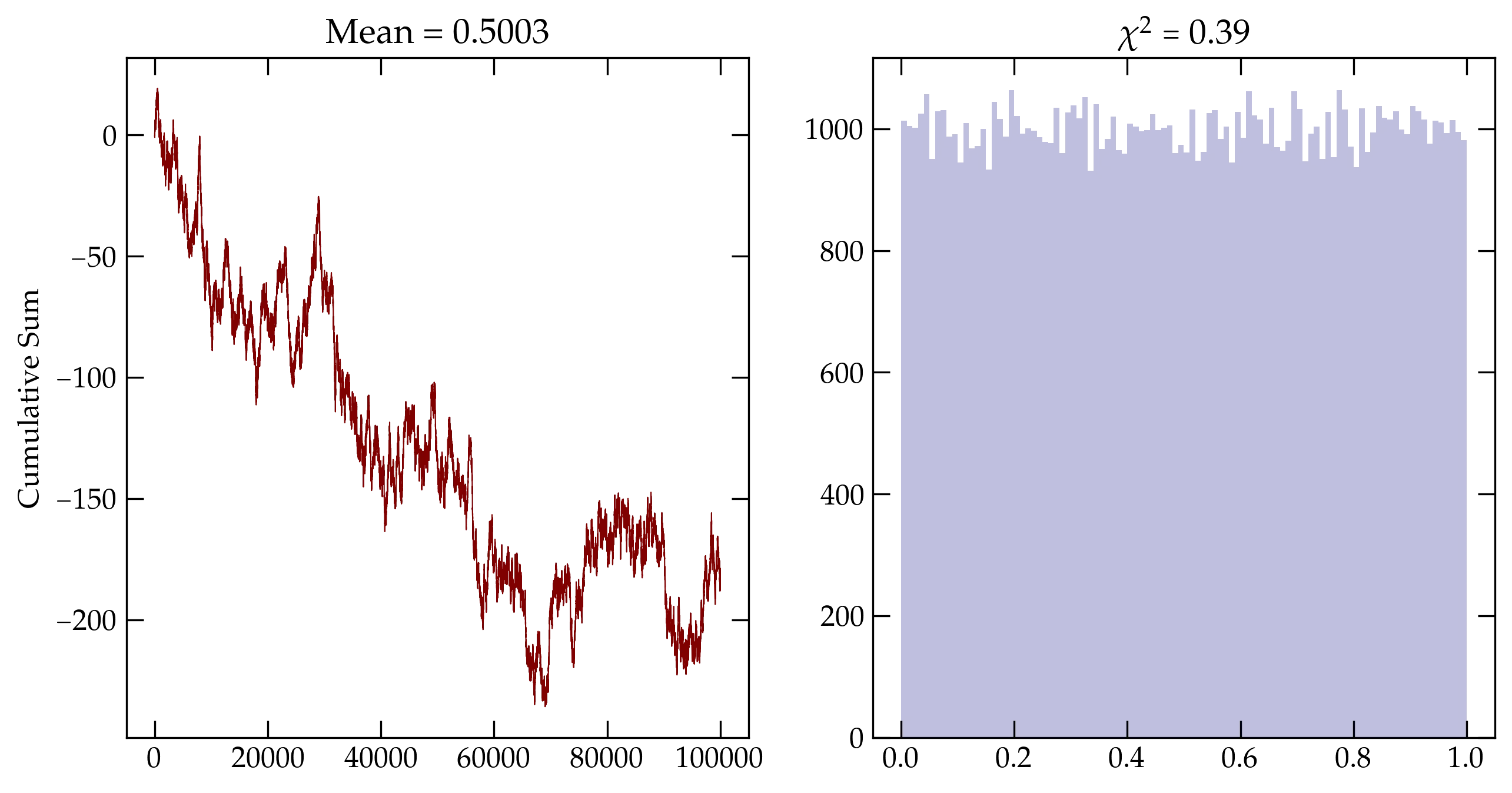
Figure 2 — Cumulative sum for a simple xorshift random number generator.
Of course, for more efficient work in Python, you should use the built-in functions:
from numpy random import default_rng

rng = default_rng() # instantiate the default random number generator
class DefRNG:
    def __init__(self, rng):
        self.rng = rng

    def uniform(self, size):
        return self.rng.uniform(size=size)

    def zero_mean(self, size):
        return self.rng.uniform(-1, 1, size=size)

test_rng(DefRNG(rng), "ST-default-rng")
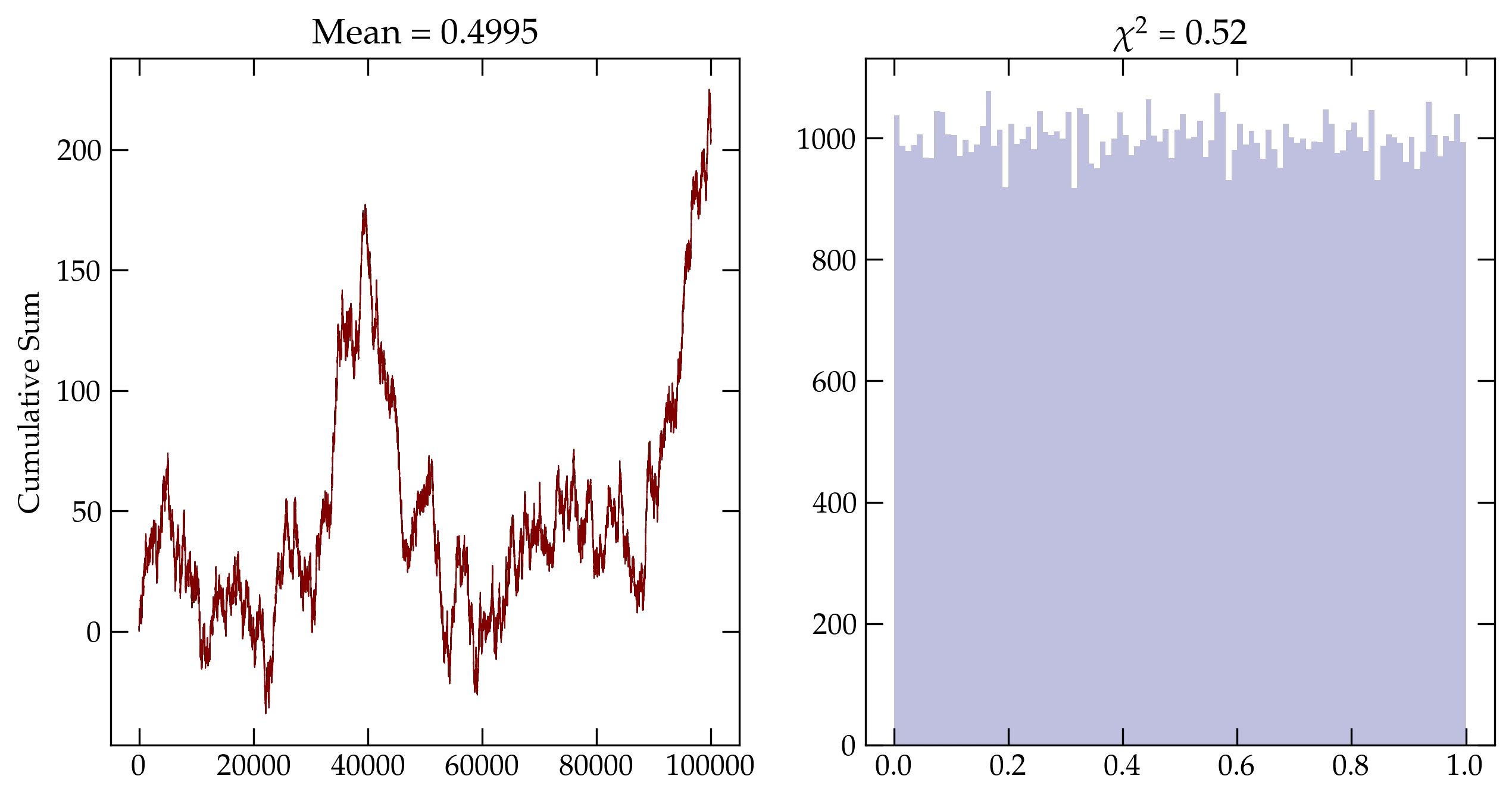
Figure 3 — Cumulative sum using numpy’s default_rng().
Sometimes you may want random numbers that follow something more exotic than a uniform distribution between 0 and 1. If, for instance you need numbers between \(-1\) and 1, you can just use 2 * rng.random() - 1. But if the distribution isn’t just a linear transformation of the range, then you have to work a bit harder. Imagine, for instance, that you draw a random number \(x\) from the range [0,1) and then apply some function \(y(x)\) to it. What is the distribution of \(y\)?
The probability that \(x\) was in an infinitesimal range of width \(\dd{x}\) around \(x\) is \(p(x)\dd{x}\). Since we start from a uniform distribution, \(p(x)\) is just a constant. That little range of \(x\) values maps into a corresponding range of \(y\) values according to \begin{equation}\label{eq:probxform} p(x)\dd{x} = P(y)|\dd{y}| \end{equation} where I need the absolute value to handle the fact that when \(x\) increases, \(y\) might decrease. Solving for the distribution \(P(y)\) gives \[ P(y) = p(x) \qty|\dv{x}{y}| = \frac{p(x)}{\qty|\dv{y}{x}|} \]
Let’s look at an example. Suppose that \(y = -\ln x\) or \(x = e^{-y}\). Then \[ P(y) = 1 \cdot |-e^{-y}| = e^{-y} \]
To illustrate this transformation, consider the following code, which computes a million uniform deviates, transforms them, and plots side-by-side histograms. The density argument to the histogram normalizes the resulting histogram to “integrate” to 1, as required for a normalized probability density distribution.
from numpy.random import default_rng
rng = default_rng()

uniform = rng.random(1000000)
expo = -np.log(uniform)
fig, axs = plt.subplots(ncols=2, figsize=(8,4))
axs[0].hist(uniform, bins=np.linspace(0,1,101), density=True)
axs[0].set_xlabel("$x$")
axs[1].hist(expo, bins=np.linspace(0,4,101), density=True)
axs[1].set_xlabel("$y$");
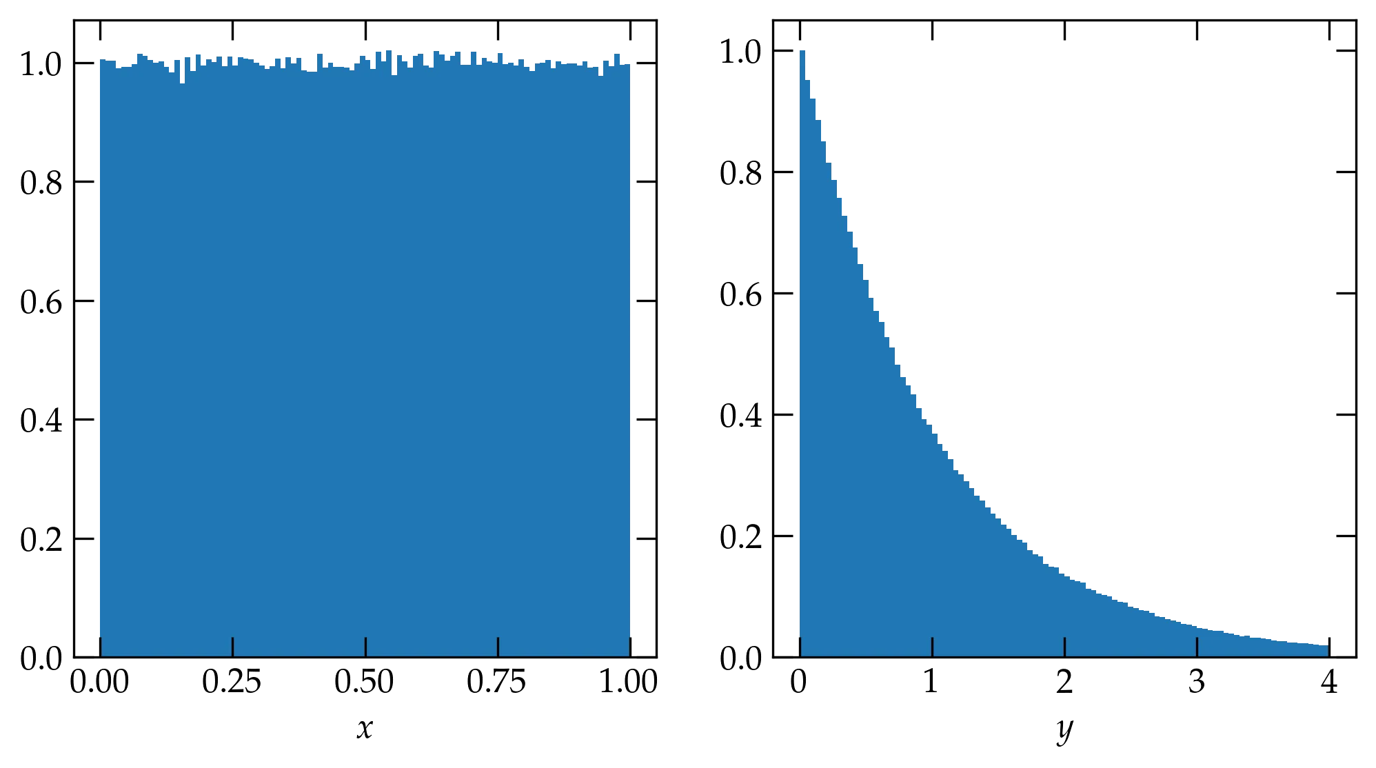
Figure 3 — Histograms of one million uniform deviates \(x\) (left) and the corresponding exponential deviates transformed via \(y = -\ln x\) (right).
One way to produce deviates that follow the normal distribution uses a generalization of Eq. \eqref{eq:probxform} to two dimensions in an approach that mimics the way Poisson and Laplace figured out how to simplify the problem by squaring it. As you perhaps learned in Math 19, the Jacobian determinant generalizes the one-dimensional transformation of Eq. \eqref{eq:probxform} to multiple dimensions: \begin{equation} \label{eq:jacobian} P(y_1, y_2, \ldots) \dd{y_1} \dd{y_2} \ldots = p(x_1, x_2, \ldots) \qty| \frac{\partial(x_1, x_2, \ldots)}{\partial(y_1, y_2, \ldots)}| \dd{y_1} \dd{y_2} \ldots \end{equation} If we let \begin{align} x_1 &= \exp\qty[-\frac12 (y_1^2 + y_2^2)] \notag \\ x_2 &= \frac{1}{2\pi} \arctan \frac{y_2}{y_1} \end{align} then the Jacobian is \[ \left|\begin{pmatrix} -y_1 e^{-(y_1^2+y_2^2)^2/2} & \frac{1}{2\pi} \frac{1}{1+y_2^2/y_1^2}\qty(-\frac{y_2}{y_1^2}) \\ -y_2 e^{-(y_1^2+y_2^2)^2/2} & \frac{1}{2\pi} \frac{1}{1+y_2^2/y_1^2}\qty(\frac{1}{y_1}) \end{pmatrix} \right| = \qty|\frac{1}{2\pi} e^{-(y_1^2+y_2^2)/2} \frac{y_1^2}{y_1^2+y_2^2}(-1 - \frac{y_2^2}{y_1^2})| = \frac{1}{2\pi} e^{-(y_1^2+y_2^2)/2} = \qty(\frac{1}{\sqrt{2\pi}} e^{-y_1^2/2}) \qty( \frac{1}{\sqrt{2\pi}} e^{-y_2^2/2}) \] That is \[ P(y_1, y_2) \dd{y_1} \dd{y_2} = \qty(\frac{1}{\sqrt{2\pi}} e^{-y_1^2/2} \dd{y_1}) \qty( \frac{1}{\sqrt{2\pi}} e^{-y_2^2/2} \dd{y_2}) \] showing that the two variables \(y_1\) and \(y_2\) each have Gaussian distributions. We now need to invert to get \(y_1\) and \(y_2\) as functions of \(x_1\) and \(x_2\): \begin{align} -2\ln x_1 &= y_1^2 + y_2^2 \notag \\ \frac{\sin(2\pi x_2)}{\cos(2\pi x_2)} &= \frac{y_2}{y_1} \notag \end{align}
So, \begin{align} y_1 &= \cos(2\pi x_2) \sqrt{-2 \ln x_1} \notag \\ y_2 &= \sin(2\pi x_2) \sqrt{-2 \ln x_1} \notag \end{align}
If we draw two numbers (\(v_1, v_2\)) at random from within the unit circle, then we can use \(r^2 = v_1^2 + v_2^2\) to find the radius, provided that it is less or equal to 1, and we can divide each by \(r\) to produce the cosine and sine values to yield two normally distributed values \(y_1\) and \(y_2\). This is the Box-Muller method.
class BoxMuller:
    def __init__(self):
        self.next = None

    def many(self, size: int):
        """
        We will likely need more than `size` random numbers from -1 to 1,
        since we can only use those whose sum of squares is ≤ 1. The fraction
        that should satisfy this condition is π / 4 ≈ 0.7854, so we should need
        something like `size` * 4 / π values
        """
        n = int(1.05 * size * 2 / np.pi)          # we'll do 5% extra
        xy = rng.uniform(-1, 1, size=(n, 2))      # fetch all the uniform deviates
        r2 = xy[:,0] ** 2 + xy[:,1] ** 2          # compute r^2
        good = np.nonzero(r2 <= 1)[0]             # which are within the unit circle?
        mag = np.sqrt(-2 * np.log(r2[good]) / r2[good])
        boxm = np.outer(mag, [1,1]) * xy[good,:]  # multiply mag by x and y
        boxy = boxm.flatten()                     # combine all the x and y deviates
        if len(boxy) >= size:                     # do we have enough?
            return boxy[:size]
        more = self.many(size - len(boxy))        # how many more do we need?
        return np.concatenate((boxy, more))

    def __call__(self, size=1):
        if size == 1:
            if self.next:
                v = self.next
                self.next = None
                return v
            while True:
                x1, x2 = rng.uniform(-1, 1, size=(2))
                r2 = x1*x1 + x2*x2
                if r2 <= 1:
                    break
            mag = np.sqrt(-2 * np.log(r2) / r2)
            self.next = x1 * mag
            return x2 * mag
        else:
            return self.many(size)

BM = BoxMuller()
v = BM(10000000)
fig, ax = plt.subplots()
ax.hist(v, bins=np.arange(-4,4,0.05), density=True);
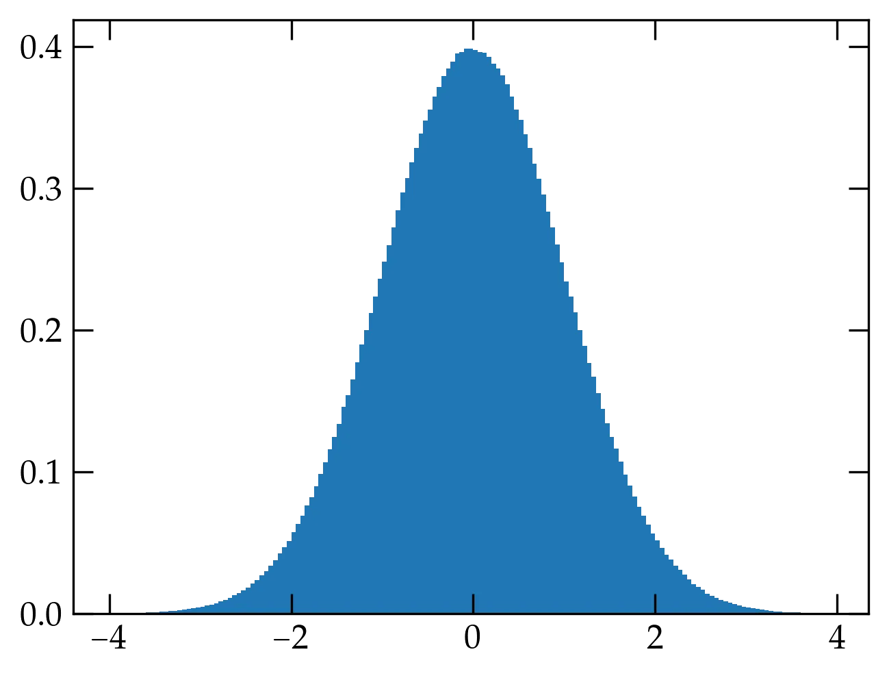
Figure 2 — Normal deviates computed using the Box-Muller method.
Naturally, NumPy has an optimized routine to generate normal deviates called rng.normal(loc, scale, size). The first two parameters are either floats or array_like of floats. The size parameter should be an int or a tuple of ints.
fig, ax = plt.subplots()
ax.hist(rng.normal(size=1000000), bins=np.arange(-4,4,0.05), density=True);
The result is essentially the same as shown above, albeit the data are computed much faster.
We have used scipy’s quad routine to perform numerical integration of a one-dimensional function; it gives both a result and an error estimate. As a reminder, we’ll compute \(\int_0^1 \tanh x \dd{x} = \ln \cosh(1)\), corresponding to the shaded area in Fig. 3.
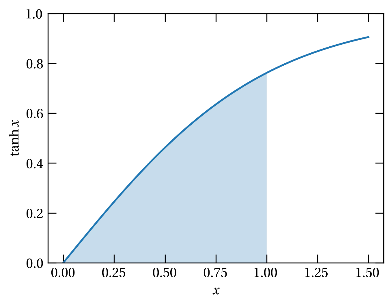
Figure 3 — Integrating under the hyperbolic tangent.
from scipy.integrate import quad
quad(lambda x: np.tanh(x), 0, 1)
(0.4337808304830271, 4.815934656432787e-15)
np.log(np.cosh(1))
0.4337808304830271
As you can see, quad worked very well indeed. Where quad may not work so well is in a multidimensional integration. If a successful evaluation of quad takes \(N\) operations, an \(n\)-dimensional integral will require \(N^n\) operations, which may take prohibitively long.
Monte Carlo integration takes an entirely different approach akin to throwing darts. To illustrate, I will compute \(\pi\) in a simple-minded way: I will throw a bunch of darts at the unit square (as in, I will draw \((x,y)\) from a random number generator that returns uniform deviates on [0,1) ). If the dart is within a radius of 1 of the origin, I will call it a success. Since the ratio of the area of the quarter circle to the square is \(\pi/4\), if I multiply the success rate by 4 I should obtain an estimate of \(\pi\).
fig, ax = plt.subplots(figsize=(9, 9))
phi = np.linspace(0, np.pi/2, 100)
ax.plot(np.cos(phi), np.sin(phi), 'k-', lw=2)
pts = rng.uniform(size=(50000,2))
r2 = pts[:,0]**2 + pts[:,1]**2
color = np.where(r2 < 1, 'g', 'r')
ax.scatter(pts[:,0], pts[:,1], s=2, marker='o', c=color)
inside = np.count_nonzero(r2<1)
pi_est = 4 * inside / pts.shape[0]
ax.set_title(r"$\pi \approx %.4f$" % pi_est);
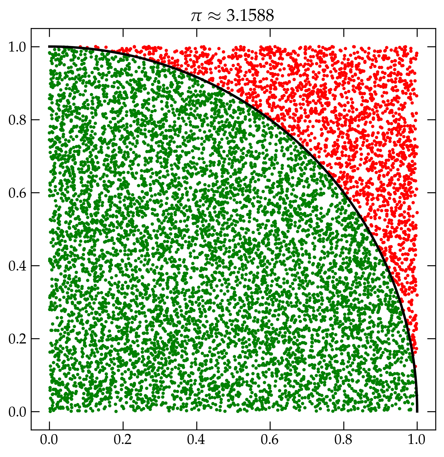
Figure 4 — Illustration of the Monte Carlo method of computing \(\pi\).
Of course, this method cannot give the exact value for the integral. How much error should we expect? If the ratio of the success area to the total is \(p\), then the probability that each dart is a success is \(p\) and the probability that it is a failure is \(q = 1 - p\). Each of the darts is independent of every other. If we throw two darts, then the four possible outcomes are the terms in \[ 1 = (p+q) (p+q) = p^2 + 2 pq + q^2 \] where the first term shows the probability of 2 successes, the second the probability of a single success, and third the probability of no successes. Generalizing to \(N\) throws, we have the probability of \(n\) successes is given by the binomial distribution. \[ P(n) = \binom{N}{n} p^n q^{(N-n)} = \frac{N!}{n! (N-n)!} p^n q^{(N-n)} \]
As derived on the binomial distribution page, the mean number of successes and their standard deviation are given by \begin{align} \ev{n} &= Np \notag \\ \sigma &= \sqrt{N p q} \notag \end{align}
Using these results, we can compute the relative uncertainty in the determination of the value of \(p\), by dividing the standard deviation of the distribution by the mean: \[ \text{relative uncertainty} = \frac{\sigma}{\ev{n}} = \frac{\sqrt{N p q}}{Np} = \sqrt{\frac{q}{Np}} \] In other words, the relative uncertainty will be minimized by making \(N\) as large as possible and \(q\) as small as possible. The latter corresponds to picking a surrounding shape that has an area as close to the success area as we can.
Of course, we know what the correct value of \(\pi\) is and our estimate is off by a relative error of \((\pi - 3.1490) / \pi = -0.002\,37\). We threw \(N = 50\,000\) darts and found \(39\,363\) inside the circle. So \(p = \frac{39\,363}{50\,000} = 0.787\,26\), which means the expected standard deviation over the mean is \[ \frac{\sigma}{\ev{n}} = \sqrt{ \frac{1-p}{Np} } = \sqrt{ \frac{1-0.787\,26}{50\,000 \cdot 0.787\,26}} = 0.002\,32 \] Very nice agreement.
The volume of a sphere is \(V = \frac{4}{3} \pi R^3\); the volume of a hypersphere in \(d\) dimensions is \(V = C_d R^d\) for some number \(C_d\) which depends on the number of dimensions. Use a Monte Carlo method to estimate \(C_5\) (obtain a value and estimate its uncertainty). Use \(N = 10^7\) points in the integration. Then compare your answer to the true answer, given by \[ C_d = \frac{\pi^{d/2}}{\frac{d}{2} \Gamma\qty(\frac{d}{2})} \]
Next: Stochastic Processes