
The purpose of the project is for you to apply the mathematical and programming skills you have been developing in the course to a computational physics problem. Given the many constraints on your time and resources, you need not aim for original research—in the sense that you need not develop a heretofore unknown method for solving a computational physics problem. Rather, the goal is for you to solve a problem consistent with your level of physics background by applying your current mastery of computational techniques, not by using the Internet to look up how somebody else has solved the problem.
I know, copying somebody else is way more efficient. After all, they already had to make a bunch of stupid mistakes, track down coding errors, and run sanity checks to gain confidence that their code actually does what they wanted it to do. Why not take advantage of their efforts? Why reinvent the wheel?
Why? Because I have high aspirations for you! I want you to be a pioneer, a developer of new knowledge, a courageous individual who can pose questions and seek answers where none already exist. Can you prepare yourself for original research by merely copying what others have figured out? I don’t think so. You have to learn how to ask and answer questions for yourself. And that’s what this project is about. So please suppress your well-honed ability to “Google the answer” and instead search within your team’s collective brains for a path to a solution.
Each team of 3 (or so) of you will develop code to simulate a system or to compute quantities of physical importance, prepare a presentation of your findings to be delivered on Wednesday, 7 May 2025 during Presentation Days, and submit your documented code in a (zip) archive by Friday, 9 May 2025. The presentations and documented code should offer a clear description of the system you are modeling, should outline choices you made in developing the code and/or refining the model, the results you have obtained, and the sanity checks you have made to confirm that your results are trustworthy.
A reference we can all share is An Introduction to Computer Simulation Methods: Applications to Physical Systems by Harvey Gould, Jan Tobochnik, and Wolfgang Christian. I will bring copies and we can copy out portions.
Some background has been added to the Stochastic page. Start there for background and for a description of the one-dimensional Ising model. A good project topic would be to generalize the model to two or three dimensions. Although there is no ferromagnetic transition of the Ising model in one dimension, there is in two or more dimensions. To get started observing the phase transition, use a modest value of \(N\) (e.g., 16) and prepare a plot of the heat capacity (per spin) as a function of temperature in the range \(1 \le T \le 3\) with \(B = 0\). You should see a peak. Theoretical considerations hold that in the limit of a large system, we expect the following behavior for the magnetization and the heat capacity \(C\) in the vicinity of the transition temperature \(T_c\), \begin{align}\label{eq:C} M(T) & \sim (T_c - T)^\beta \qquad T < T_c \notag \\ C(T) & \sim |T - T_c|^{-\alpha} \notag \\ \chi(T) & \sim |T - T_c|^{-\gamma} \end{align} where \(\alpha\) and \(\gamma\) are called critical exponents. For the two-dimensional Ising model, \(\beta = 1/8\) and \(\gamma = 7/4\); in three dimensions, they are \(\beta = 0.32\) and \(\gamma = 1.24\). How closely can you determine \(T_c = 2 / \ln(1 + \sqrt{2})\)? See Chapter 15 of Gould, Tobochnik, and Christian, An Introduction to Computer Simulation Methods for lots more information and project ideas, including putting a two-dimensional array of spins on a triangular lattice, rather than a square lattice.
Chapter 16 discusses many approaches to simulating quantum systems. You may have explored the shooting method for finding eigenstates of the “quark potential”, \(V \sim \|x\|\). Does this approach generalize to higher spatial dimensions? Does it depend on having rotational or other symmetry that allows the problem to be factored?
Chapter 10 discusses numerical solutions to boundary value problems, including Gauss-Seidel relaxation. Are there more direct methods that start from the same premise of a finite difference approximation to the Laplacian operator?
Chapter 8 discusses the dynamics of many-particle systems (often called molecular dynamics). We assume that the particles interact with one another via a known potential energy function, such as the Lennard-Jones potential, \begin{equation}\label{eq:Lennard-Jones} U(r) = 4 \epsilon \qty[ \qty(\frac{r_0}{r})^{12} - \qty(\frac{r_0}{r})^6] \end{equation} \(r\) is the distance between the two particles, \(\epsilon\) is the depth of the attractive portion of the potential, and \(r_0\) is the value of \(r\) at which the two terms in brackets are equal and so \(U(r_0) = 0\). By taking the gradient of the potential, you can find the force on each of the two particles. Dividing by the appropriate mass then gives you the contribution to the acceleration of each particle caused by this interaction. You must then sum these accelerations over all pairs of particles to determine how to update the particle positions and velocities.
Once you have determined the acceleration of all the particles, you can then update their positions and velocities using the velocity Verlet algorithm: \begin{align} x_{n+1} &= x_n + v_n \Delta t + \frac12 a_n (\Delta t)^2 \label{eq:pos-update} \\ v_{n+1} &= v_n + \frac12 (a_{n+1} + a_n) \Delta t \end{align} A few considerations are in order:
For \(N\) particles, the number of pairs is \(N(N-1)/2\). Typically, you don’t have to evaluate all of them; the force dies off very rapidly for distances beyond something like \(2 r_0\). Nonetheless, a straightforward implementation requires that you analyze \(N(N-1)/2\) pairs (some of which you may simplify to zero if the particles are far enough apart). Therefore, the computational time to evaluate the accelerations scales as \(N^2\). When the number of particles is small, this is not a big problem. For large simulations, however, the \(N^2\) dependence can really slow things down. The Barnes-Hut algorithm is an approach to sorting the particles that lowers the number of operations needed to compute the accelerations from \(O(N^2)\) to \(O(N \log_2 N)\) using octrees.
More project ideas are described and illustrated on this page.
I’m going to go way out on a limb and suggest that you started the project with confusions, misunderstandings, and uncertainty about where you were headed or downright ignorance of the system you chose. I will further speculate that as you worked on it, you made some false moves, explored some dead ends, and gradually came to appreciate what worked and what didn’t. There are two key points about this journey:
Invite us to learn with you, tracing for us the most useful path through the conceptual minefield so we are led to enlightment without having to spend as much time as you did.
The advice “why before how” also applies to individual slides, if you make them.

Figure 1 — This is a visually appealing slide created by a clinic team that aimed to explain how they were using a technique called dynamic light scattering to determine the size of particles in their samples. The title, “Dynamics Light Scattering” identifies the technique they used. They knew nothing about DLS at the start of the project and most audience members know nothing about it. Can you think of a more helpful title?
Rather than titling a slide with the name of the phenomenon or technique, consider using a question, as illustrated in Figure 2.
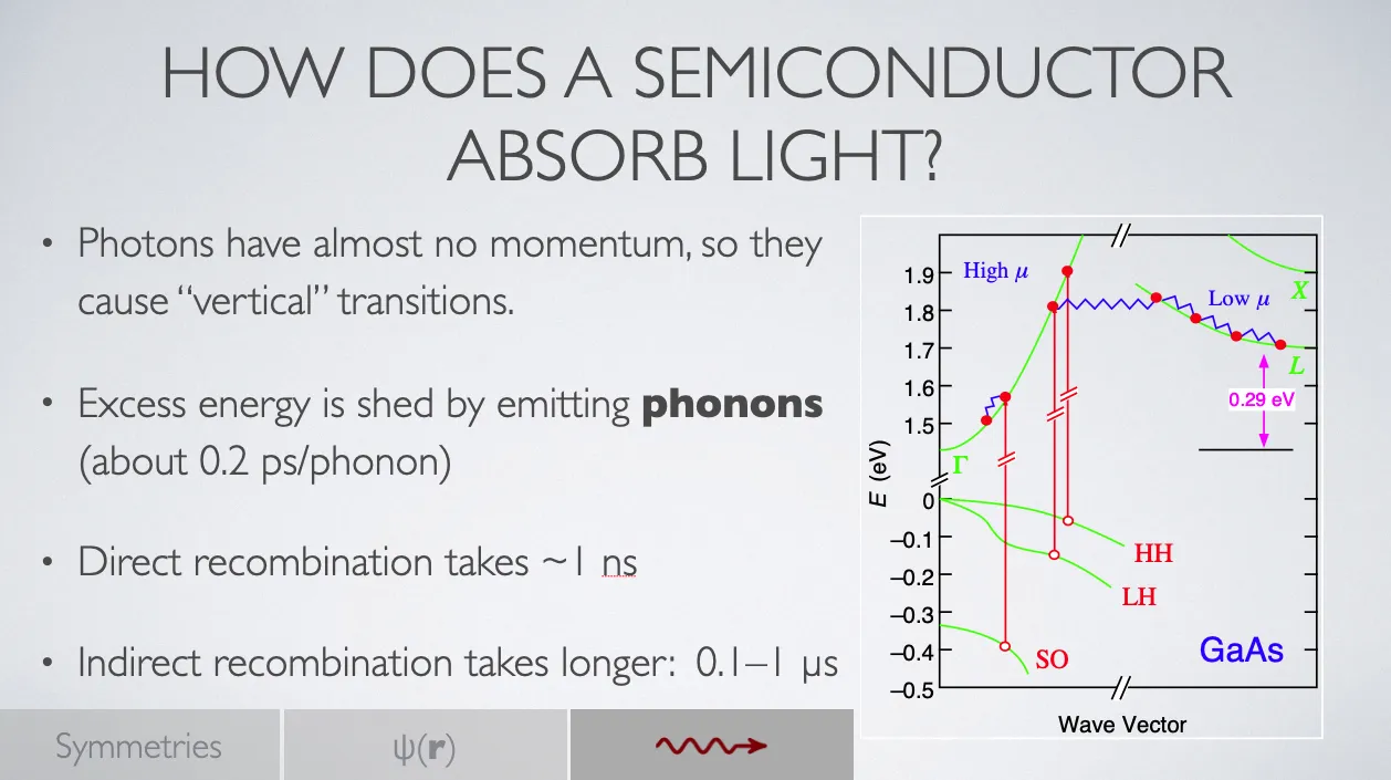
Figure 2 — I could have titled this slide “Interband Transitions”, which makes perfect sense to those already in the know. However, I think using a question that gets at the heart of the issue is more helpful. My title for Fig. 1 might be “How We Measure Particle Size”.
As the presenter, you know (should know?) more about your topic than the audience does. Your goal should not be to lord this superiority over them, but to invite them to learn something interesting about the topic you have studied and in which you have developed expertise.