
Computation in this course will use Python and JupyterLab, which are open-source software that is free to install and use. You are responsible for making sure that you have a working setup on your personal computer; I offer here some guidance.
python.> python
Python 3.14.2 (main, Dec 5 2025, 16:49:16) [Clang 17.0.0 (clang-1700.4.4.1)] on darwin
Type "help", "copyright", "credits" or "license" for more information.
>>>
> wsl -l -v
If WSL is not installed, you can install it with
> wsl --install
Once you have installed WSL, you need to create a user account and password for your newly installed Linux distribution. Follow the instructions on the WSL page. Then skip to the instructions below for installing on Ubuntu (Linux).
You may already have installed on your computer all the software you need for this course. To check, run the following code. If it generates the plot, you are ready to proceed to Jupyter.
import numpy as np
import matplotlib.pyplot as plt
import pandas as pd
from numpy.random import default_rng
rng = default_rng()

x = np.arange(0, 10, 0.1)
y = np.exp(np.sqrt(x))
noise = rng.normal(size=len(x))
fig, ax = plt.subplots()
ax.plot(x, y)
ax.plot(x, y + noise, 'r.')
ax.set_xlabel("$$x$$", usetex=True)
ax.set_ylabel(r"$$y = e^{\sqrt{x}}$$", usetex=True)
ax.set_title("Did it work?")
plt.show()
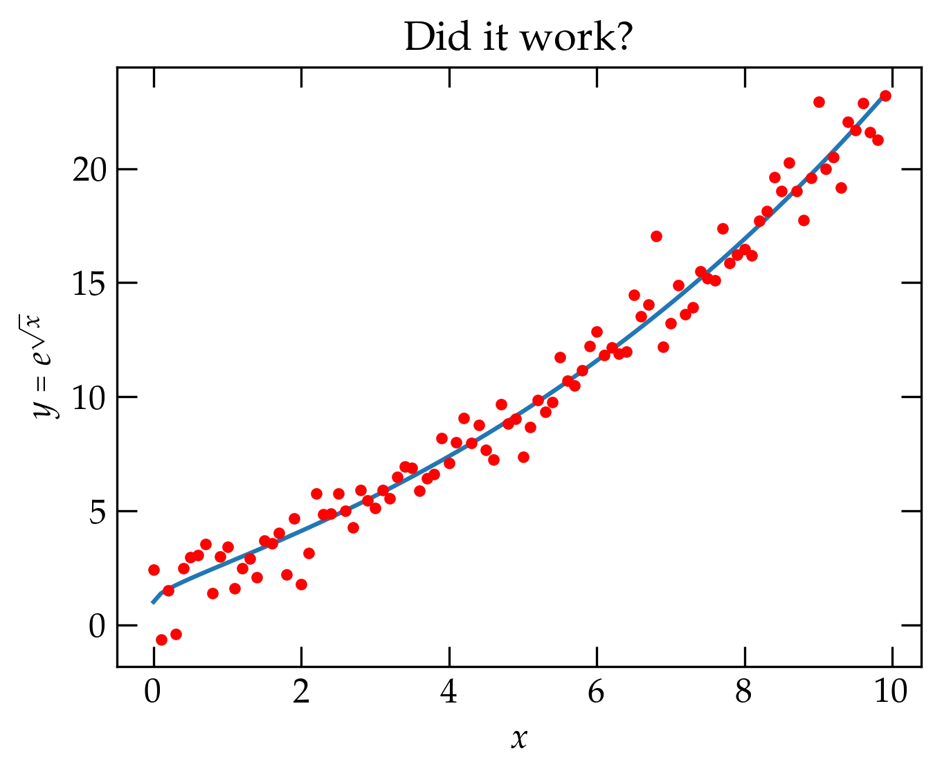
Figure 1 — Copy the code above and run it in a terminal after launching Python. If it generates this graph, you have all the packages we’ll need.
The computational portions of the course will use Python 3 and several modules,
most notably numpy, scipy, and matplotlib, and jupyter. If you are starting from scratch, I recommend you just install the Jupyter Lab application:
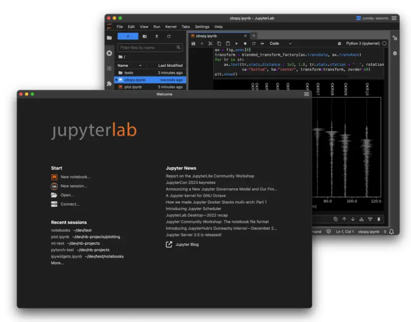
Figure 1 — Installing the JupyterLab Desktop Application
Head to its GitHub repository, then scroll down the page until you get the Installation section.
Click the link that corresponds to your operating system and processor.
Follow installation instructions, and read carefully any messages.
When you have finished installing, launch the Jupyter Lab application and watch whether it reports that you need to identify a Python installation. If it does, it gives you a link to install a default Python. Do that! It takes a bit longer, but once it’s done, you have everything you need. It installs numpy, scipy, matplotlib, ipython, and ipympl. To check your installation, click the New notebook… link on the jupyterlab homepage and enter the following in the cell:
import numpy as np
import matplotlib.pyplot as plt
%matplotlib widget

fig, ax = plt.subplots()
ax.plot([1, 2], [3, 4], 'ro')
Press shift-return to execute the code in the cell. If your installation is working properly, you should see a really dumb plot with two red dots:
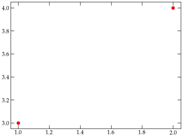
Figure DP — a dumb test plot.
If you have Anaconda installed, you may already have everything you need. However, I prefer
not to use Anaconda, but to install the tools I need using pip, the Python
installer program.
Alternatively, you can let Google take care of hosting the software (which, of course, requires a live net connection) by using Google Colab, a Google-inflected version of JupyterLab. If you use this approach, all you need to do is head to Google’s colab page. If you need to access your own Python code, see the Colab page for more information.
An Anaconda installation should already have Jupyter notebook installed and available, but you don’t need the full Anaconda distribution to use Jupyter notebook and I have had some trouble in the past getting Anaconda to update to a more recent version of some of the tools. If you already have an Anaconda installation, it seems reasonable to check it out and make sure that it can run what we need. Otherwise, I highly recommend a light-weight approach using Python/Pip, as described below.
If you have Anaconda installed you can launch the Anaconda Navigator from which you can launch Jupyter notebook. You can download Anaconda from https://www.anaconda.com/.
Many systems have Python installed automatically. At this point, there is no
reason to use Python 2.7.x; it has been deprecated and is no longer supported
(although many projects have stubbornly refused to update to Python
3). Because Python 2 still hangs around, typing python at a command prompt
may launch a version 2 interpreter. You can test with
> python
Python 2.7.17 (default, Dec 23 2019, 21:25:33)
[GCC 4.2.1 Compatible Apple LLVM 11.0.0 (clang-1100.0.33.16)] on darwin
Type "help", "copyright", "credits" or "license" for more information.
>>>
To be sure that you are running some flavor of Python 3, you can use python3:
> python3
Python 3.13.1 (main, Dec  3 2024, 17:59:52) [Clang 16.0.0 (clang-1600.0.26.4)] on darwin
Type "help", "copyright", "credits" or "license" for more information.
>>>
If you have a much older version of Python 3 than the one listed above, it is probably worthwhile upgrading to the current version.
Although there is a Python version already installed in MacOS, it tends to lag
behind and I much prefer to use Homebrew to install an up-to-date version of Python (and plenty of other free software). You can check if you already have it installed by opening up a terminal window (the Terminal.app program is in /Applications/Utilities/Terminal.app, or you can use an alternative terminal
program, such as iTerm2).
> which brew
/opt/homebrew/bin/brew
Since I already have the brew command installed, I see that it is located in
/opt/homebrew/bin, which is where most Homebrew commands get linked.
If you do not have Homebrew installed, you can follow the directions at brew.sh or paste the following at the terminal.
/bin/bash -c "$$(curl -fsSL https://raw.githubusercontent.com/Homebrew/install/HEAD/install.sh)"
Once Homebrew is installed, use it to install python:
brew install python
This should install the most recent stable version of Python 3. It also includes
the Python installer pip.
> brew --version
Homebrew 5.0.8
I strongly recommend installing Windows Subsystem for Linux, which gives you a UNIX command line and all the utilities you need to run Python, pip, etc. You can check whether WSL is installed by typing the following command into PowerShell or the Windows Command Prompt:
> wsl -l -v
If WSL is not installed, you can install it with
> wsl --install
Once you have installed WSL, you need to create a user account and password for your newly installed Linux distribution. Follow the instructions on the WSL page. Then skip to the instructions below for installing on Ubuntu (Linux).
Download the Anaconda3 installer and launch it. After it finishes installing, launch the Anaconda Navigator. Then click to launch a Powershell:
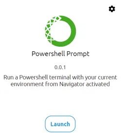
This opens a terminal window. Enter the command
pip install ipympl
to install the Python package that allows graphs generated by Matplotlib to be
displayed inside a jupyter lab window.
Make sure that Python 3 is installed:
sudo apt update
sudo apt -y upgrade
sudo apt install -y python3-dev python3-pip
sudo apt install -y build-essential libssl-dev libffi-dev
You can learn a lot about your current environment by issuing the env command
at a terminal prompt:
> env | sort
COLORTERM=truecolor
COMMAND_MODE=unix2003
EDITOR=/Applications/Emacs.app/Contents/MacOS/Emacs
GEM_HOME=/Users/saeta/.gem
HOME=/Users/saeta
ITERM_PROFILE=Default
LANG=en_US.UTF-8
LC_TERMINAL_VERSION=3.6.6
LC_TERMINAL=iTerm2
LOGNAME=saeta
LSCOLORS=exfxcxDxbxegeDabagacadah
OMF_CONFIG=/Users/saeta/.config/omf
OMF_PATH=/Users/saeta/.local/share/omf
PATH=/Users/saeta/.virtualenvs/py14/bin:/Users/saeta/bin:/Users/saeta/.juliaup/bin:/usr/local/bin:/usr/local/sbin:/opt/homebrew/bin:/opt/homebrew/sbin:/opt/local/bin:/Users/saeta/Library/Python/3.10/bin:/opt/homebrew/opt/ruby/bin:/Users/saeta/.pyenv/bin:/opt/homebrew/opt/fzf/bin:/usr/local/bin:/System/Cryptexes/App/usr/bin:/usr/bin:/bin:/usr/sbin:/sbin:/var/run/com.apple.security.cryptexd/codex.system/bootstrap/usr/local/bin:/var/run/com.apple.security.cryptexd/codex.system/bootstrap/usr/bin:/var/run/com.apple.security.cryptexd/codex.system/bootstrap/usr/appleinternal/bin:/opt/pmk/env/global/bin:/Library/Apple/usr/bin:/Library/TeX/texbin:/Applications/Wireshark.app/Contents/MacOS:/Users/saeta/Applications/iTerm.app/Contents/Resources/utilities:/Users/saeta/.local/bin:/Users/saeta/.gem/ruby/3.4.0/bin:/usr/local/mysql/bin:/Users/saeta/.hishtory
PGPORT=5432
PWD=/Users/saeta/Documents/Courses/p064/2025
PYENV_ROOT=/Users/saeta/.pyenv
PYTHONPATH=/Users/saeta/.python
SHELL_PID=52198
SHELL=/opt/homebrew/bin/fish
SHLVL=1
TERM_PROGRAM_VERSION=3.6.6
TERM_PROGRAM=iTerm.app
TERM=xterm-256color
USER=saeta
VIRTUAL_ENV=/Users/saeta/.virtualenvs/py14
In particular, notice the value of the PATH shell variable, which tells you
where the system will look for commands that you name on the command line, and
shows them in the order in which they will be searched. Paths are separated with
colons, so in this example, my shell will first look in /Users/saeta/.virtualenvs/py14/bin, then
in /Users/saeta/bin, etc. If you have installed Anaconda, your PATH variable may
start with the path to the bin directory inside your Anaconda distribution.
Python has a standard package manager, pip, which stands for Package
Installer for Python. You can check if pip is available by entering the
following command at a terminal prompt:
$$ pip --version
pip 25.3 from /Users/saeta/.virtualenvs/py14/lib/python3.14/site-packages/pip (python 3.14)
Look carefully at the path to your version of pip. If it has Anaconda in it somewhere, then it is associated with an existing Anaconda installation (perhaps a relic from CS 5?) and likely for an older version of Python and Pip. If so, see if you can upgrade to a current version of Anaconda and its associated versions of numpy, scipy, matplotlib, and plotly.
If the pip command doesn’t work, try running the following command to see where Python packages are being installed:
python -c "import site; print(site.getsitepackages())"
If you have a Python 3 installation, and pip is available, you can install everything you need with the following. I recommend that you can first create a virtual environment for this Python installation
so any upgrades or installed libraries don’t encounter conflicts. The following commands show how to create a virtual environment named py14:
$$ pip install --user virtualenv   # install virtualenv
$$ python -m virtualenv py14       # the standard virtualenv package
After creating the virtual environment above, you need to activate it. Check the output of the previous command to see where your virtual environment is located.
On my installation, virtual environments are located in $HOME/.virtualenvs/. So, the py14 environment is located at /Users/saeta/.virtualenvs/py14. Within that directory there is a bin directory that holds scripts and binary (executable) files. If I were located within the py14 directory, I would then run
$$ source bin/activate.sh
to activate the py14 virtual environment. Once you have activated your virtual environment (which you can check with the env command described above), run
pip install --upgrade pip  # make sure you have an up-to-date version
pip install numpy scipy matplotlib jupyter pandas
These commands install the minimum you need to get going. However, I recommend also installing some more packages:
pip install autopep8 ipympl plotly
jupyter contrib nbextension install --user
Although Jupyter and Matplotlib work “out of the box,” you will probably want to customize things a bit. Here are some basic ideas.
First install jupyter_contrib_nbextensions from pip:
pip install jupyter_contrib_nbextensions
Next install the necessary javascript and css files
jupyter contrib nbextension install --user
pip install jupyter_nbextensions_configurator
jupyter nbextensions_configurator enable --user
Launch Jupyter notebook from the directory where you would like to load code and save notebooks:
> cd ~/Documents/testing
> jupyter notebook
A browser window should open and you will see a listing of the files in the current directory. At the bottom of the Edit menu you should see
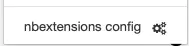
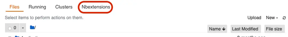
You should now see a menu item called Nbextensions, as illustrated in the figure.
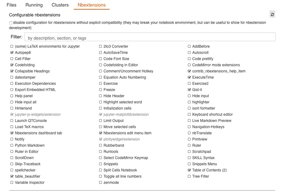
Clicking on the Nbextensions menu will allow you to load extensions as desired. I recommend several, including
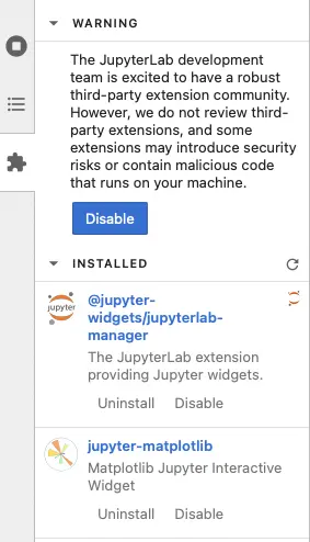
We will need a couple of extensions to be installed in JupyterLab. The first step to install those is to enable them by clicking the jigsaw icon as shown in the figure below and then clicking on the Enable button.
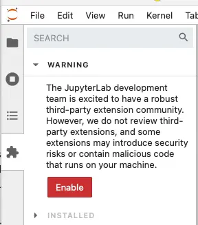
Once you have enabled extensions, you can use the search box to install the two extensions shown here
Alternatively, you can issue the following statement in the terminal
jupyter labextension install @jupyter-widgets/controls @jupyter-widgets/jupyterlab-manager \
   jupyterlab-plotly jupyter-matplotlib
By default, Jupyter notebook uses a fixed-width column no matter how wide you make your browser window. Perhaps this is just what you want, but I have sometimes found it very convenient to allow the column to expand with the window.
You can override default styling of notebook cells by preparing a custom.css
file and placing it in ~/.jupyter/custom/custom.css. The following example
allows the width of the cell to expand as the window is made wider:
.container {
  width: 100% !important;
  margin-right: 40px;
  margin-left: 40px;
}
I dislike matplotlib’s defaults. Although it is possible to customize each plot,
it is convenient to put common changes in a preferences file. A copy of the
format file is located in site-packages/matplotlib/mpl-data/matplotlibrc. Save
a copy of this file at ~/.config/matplotlib/matplotlibrc on a Unix/Linux
system or in $$HOME/.matplotlib/matplotlibrc on other systems.
This file has all sorts of options, all of them commented out with leading hash tags. Uncomment the lines you wish to modify and set appropriate values. On my system, I have set the following lines:
saeta@Saeta-MBP19~/.c/matplotlib> grep "^[^ #]" matplotlibrc
backend             : macosx
font.family         : serif # sans-serif
font.size           : 12.0 # 10.0
font.serif          : Utopia, DejaVu Serif, Bitstream Vera Serif, ...

text.usetex         : True ## use latex for all text handling.

xtick.top           : True ## draw ticks on the top side
xtick.direction     : in   ## direction: in, out, or inout
ytick.right         : True ## draw ticks on the right side
ytick.direction     : in   ## direction: in, out, or inout

savefig.format      : pdf  ## png, ps, pdf, svg
savefig.transparent : True ## setting that controls whether figures are saved with a
                           ## transparent background by default
If you set text.usetex: True in the configuration file, you can take full
advantage of TeX formatting in labels and annotations. However, beware that
certain characters that have special meaning in TeX, such as the underscore, may
cause labels to throw TeX errors unless they are in math mode. If you have
set the default text style to use TeX, you can always pass the optional
keyword argument usetex=False in the label to avoid the problem.
You can change the defaults used to generate graphs in a notebook by writing
values directly to the matplotlib.rcParams dictionary.
import matplotlib as mpl
mpl.rcParams['figure.figsize'] = [12, 8] # You can adjust the plot size
mpl.rcParams['axes.titlesize'] = 18
mpl.rcParams['axes.labelsize'] = 14
mpl.rcParams['xtick.labelsize'] = 14
mpl.rcParams['ytick.labelsize'] = 14
mpl.rcParams['legend.fontsize'] = 'large'
If you’d like to see all the available parameters and their current values, launch Python and run
import matplotlib as mpl
for k, v in mpl.rcParams.items():
    print(f"{k: >32s} = {v}")
The output runs to 300+ lines.