
Jupyter(lab) notebooks provide an interactive computation and authoring environment that allows one freely to combine text (including LaTeX equations), graphics, computation, and the results of computations in a single window. Jupyter Notebook was the original platform, but has now been superseded by Jupyterlab. My preferred approach is to use the stand-alone Jupyter Lab application.
Notebook cells can include text written in Markdown (such as this cell), Code (the cell below this one) or Raw mode. Markdown cells can include formatting information and math expressions written in LaTeX (more about that in a bit). Raw cells just hold the text and don’t interpret symbols that would change the font or show equations if they were processed as Markdown. Code cells get submitted to the Jupyter kernel (and passed to the Python interpreter). This cell is in Raw mode so I can illustrate the basics of Markdown.
Italics: *this will be in italics*

Boldface: **whereas this statement is in boldface.**

Code: `def fred(x, y)`

- a bullet
- in a list

1. Or a numbered
2. list

To write math, surround with dollar signs:
$E = m c^2$ or $x = \frac{-b \pm \sqrt{b^2 - 4 a c}}{2a}$

To center an equation on its own line, use
\begin{equation}
\sin^2 \theta + \cos^2 \theta = 1
\end{equation}

Notice that mathematical functions should be preceded with a backslash
and that you get Greek letters by preceding their name in English with a backslash.

For more information about Markdown, check out the **Markdown Reference**
item in the Jupyter **Help** menu.
And this is how that same text appears when used in a Markdown cell:
Italics: this will be in italics
Boldface: whereas this statement is in boldface.
Code: def fred(x, y)
To write math, surround with dollar signs: \(E = m c^2\) or \(x = \frac{-b \pm \sqrt{b^2 - 4 a c}}{2a}\)
To center an equation on its own line, use \begin{equation} \sin^2 \theta + \cos^2 \theta = 1 \end{equation}
Notice that mathematical functions should be preceded with a backslash and that you get Greek letters by preceding their name in English with a backslash.
For more information about Markdown, check out the Markdown Reference item in the Jupyter Help menu.
The first step in a new notebook is typically a cell that loads the modules you need and contains a magic command to specify how to render graphics. containing a magic command that allows graphs to appear in output cells of the notebook. Magic lines start with a % (and you can’t put a comment after them the way you can in Python. To execute the commands in a cell, make sure the cell is selected and press shift-enter or shift-return. Or, if you are a mouse person, click the triangle symbol at the top of the page.
# the following line is for jupyterlab
%matplotlib widget
# if you use jupyter notebook, replace "widget" with "notebook"
import numpy as np               # np is the standard abbreviation for numpy
import matplotlib.pyplot as plt  # plt is the standard abbreviation for pyplot
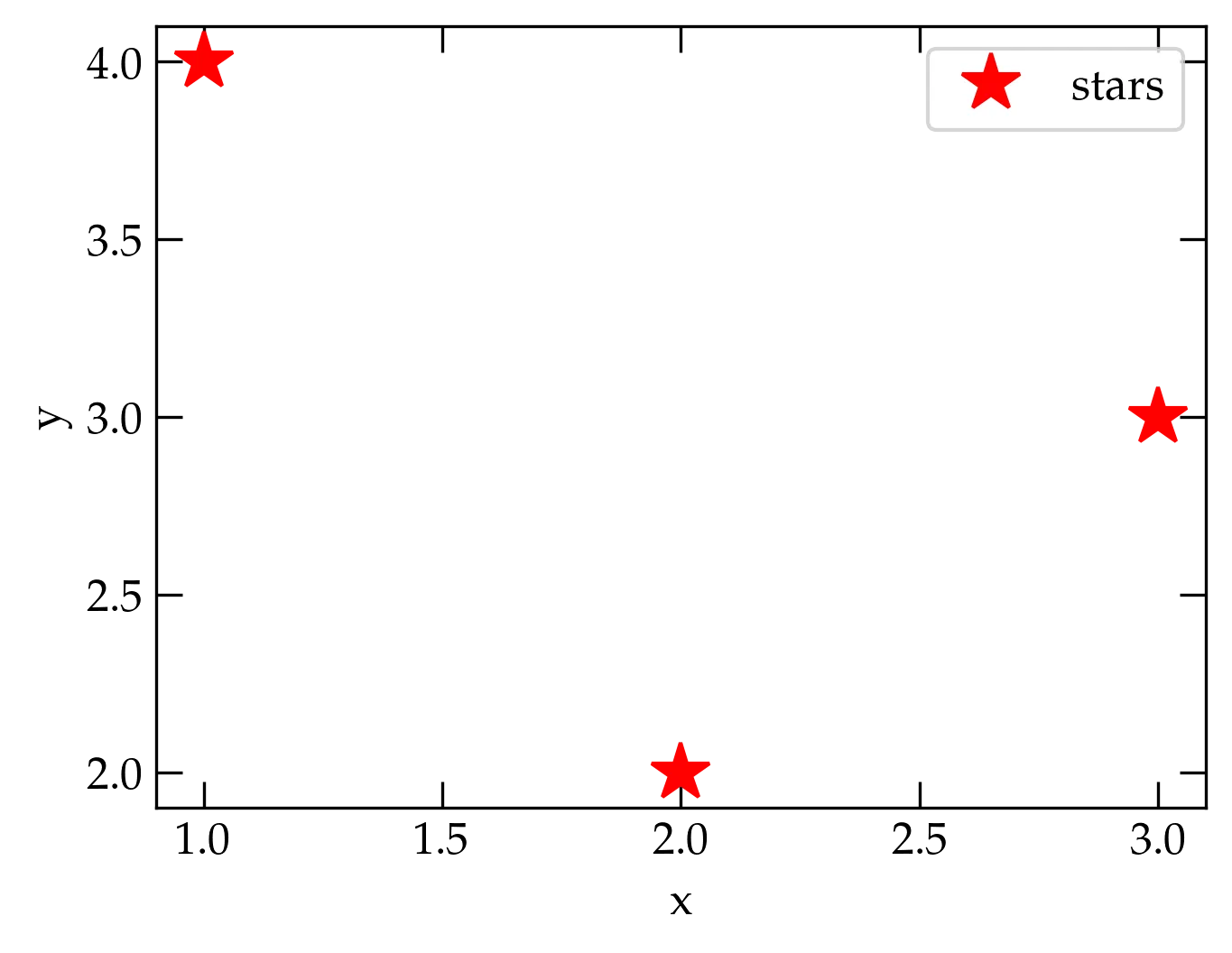
To illustrate how you can make a plot and have it show up in the notebook, let’s try a very simple example.
fig, ax = plt.subplots()
ax.plot([1, 2, 3], [4, 2, 3], 'r*', ms=16, label="stars")
ax.set_xlabel("x")
ax.set_ylabel("y")
ax.legend();
Some explanations:
plt.subplots returns both a figure object and an axes objectax.plot takes two lists, one for the x values, and the other for the y
values. They must have the same length! The optional argument 'r*' says to use
red star symbols, ms=16 sets the marker size, and the label allows the legend to associate a label with
the symbol in the legend.ax.set_xlabel and ax.set_ylabel take a string. The string can contain
LaTeX commands (see below).ax.legend(); says to show a legend of the traces on the plot, letting
matplotlib decide the best location for it. The semicolon suppresses the
output of this command. (You can remove it and run the command again to see
what gets returned.)See Introduction to Matplotlib for some basics on using Matplotlib to generate plots.
For Jupyter Lab to work with matplotlib, you need to have a few extensions installed. If plotting or animations aren’t working for you, you may have out-of-date versions of Python and/or the necessary modules.
From a terminal, type
> jupyter labextension list
JupyterLab v4.3.4
/Users/saeta/.virtualenvs/py13/share/jupyter/labextensions
        anywidget v0.9.13 enabled OK
        jupyterlab_pygments v0.3.0 enabled OK (python, jupyterlab_pygments)
        jupyter-matplotlib v0.11.6 enabled OK
        spreadsheet-editor v0.7.2 enabled OK (python, jupyterlab-spreadsheet-editor)
        jupyterlab-execute-time v3.2.0 enabled OK (python, jupyterlab_execute_time)
        @jupyter-notebook/lab-extension v7.3.2 enabled OK
        @voila-dashboards/jupyterlab-preview v2.3.8 enabled OK (python, voila)
        @jupyter-widgets/jupyterlab-manager v5.0.13 enabled OK (python, jupyterlab_widgets)
This command gives the version of the JupyterLab software and the status of all installed and enabled extensions. I have found that I need both @jupyter-widgets/jupyterlab-manager and jupyter-matplotlib installed and enabled. See below for instructions on installing and updating them right from within Jupyter Lab.
Notice that my installation is in the /opt/homebrew directory structure, since I installed it with homebrew. If your installation is from anaconda, which you can tell by looking at the directory path of the files listed in the output you see from the jupyter labextension list command, then please try
conda update conda
conda update anaconda
Kate Riggs found that these two commands fixed her installation, which was running an old version of Python and which would not display figures.
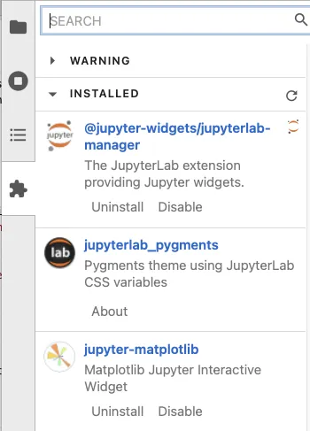
Extensions may be installed using the Extension Manager, at the bottom of the View menu. Near the top of the PyPi panel is a Warning section. You will have to grant permission to allow third-party extensions to be installed. You only have to do this once.