
An infinite series is an infinite sum, \begin{equation}\label{eq:infseries} S = \sum_{n=1}^{\infty} a_n = \lim_{N\to\infty} \sum_{n=1}^N a_n \end{equation} that is the limit of partial sums having a finite number of terms. For the limit to exist, the magnitude of the terms \(a_n\) must go to zero as \(n\to\infty\). However, while this is a necessary condition it is not sufficient. Series are among the most important mathematical tools in the physicist’s toolbox. You are no doubt already familiar with Taylor series; for problems that are difficult to solve exactly, we can often satisfactory approximations by truncating a Taylor series. For example, the equation of a simple pendulum is \[ \dv[2]{\theta}{t} + \frac{g}{L} \sin\theta = 0 \] It is a nonlinear differential equation because the variable \(\theta(t)\) appears as a nonlinear function. That is \[ \sin \theta = \theta - \frac{\theta^3}{3!} + \frac{\theta^5}{5!} - \cdots \] includes terms with higher powers of \(\theta\) than the first. However, if we ignore all terms but the first in the Taylor series for \(\sin\theta\), we obtain \[ \dv[2]{\theta}{t} + \frac{g}{L} \theta = 0 \] which is the equation of a simple harmonic oscillator and has a solution we can readily compute.
Key issues we need to understand include:
The harmonic series, \[ H = \sum_{n=1}^{\infty} \frac1n = 1 + \frac12 + \frac13 + \cdots \] does not converge, even though its terms tend to zero as \(n \to \infty\). Its divergence is logarithmic (i.e., weak), as illustrated in the following figure
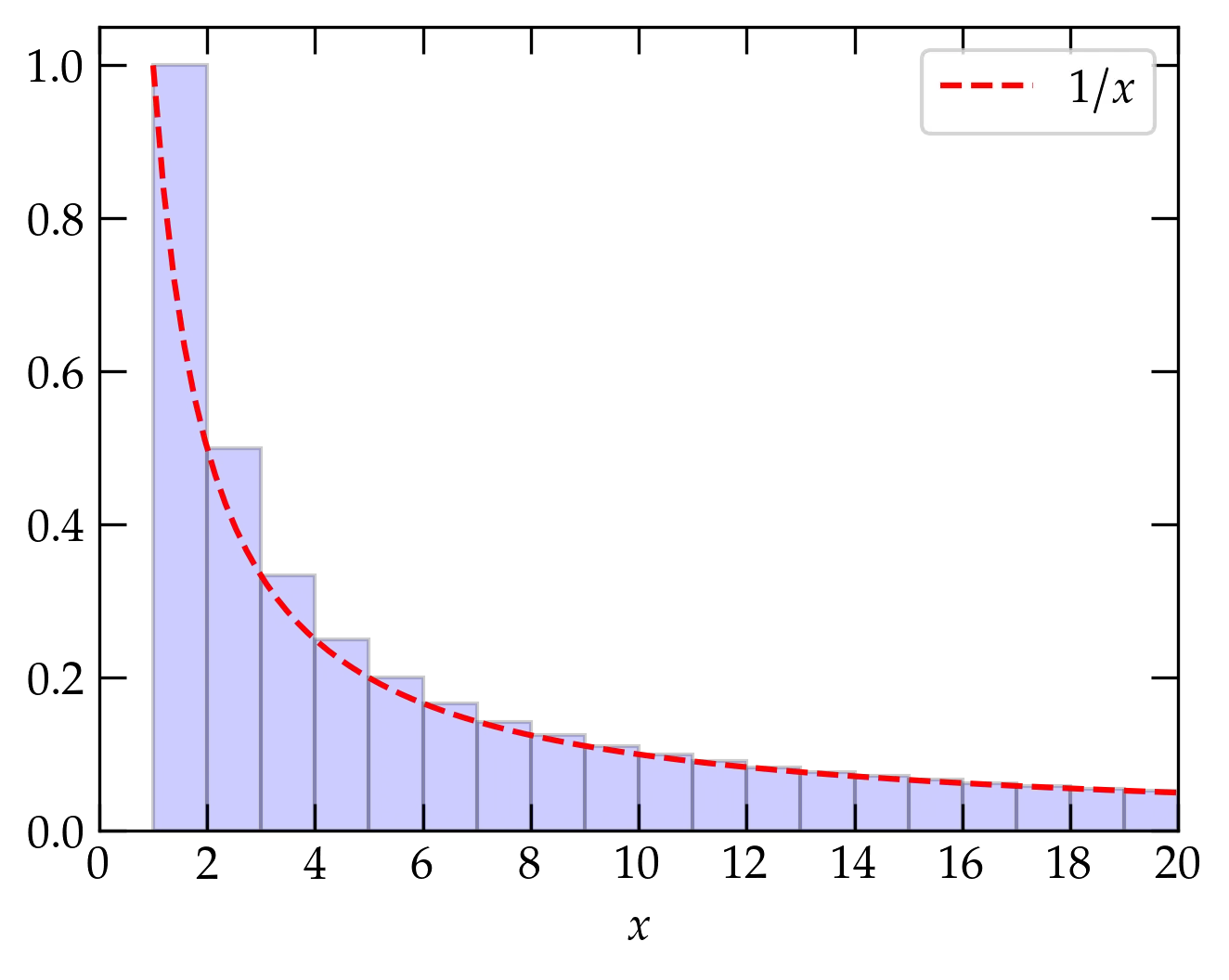
Figure 1 — The harmonic series is represented by the area shaded blue of the bars of height \(1\), \(\frac12\), \(\frac13\), etc. The area of the bars is greater than the area under the curve \(1/x\) (shown in red), since the curve is everywhere contained within a bar. Since \(\int_1^x \frac1{x'}\dd{x'} = \ln x\), which slowly diverges as \(x\to\infty\), the harmonic series diverges even though its individual terms tend to zero.
Successive terms of a geometric series form a fixed ratio \(r\): \[ S_N = a_0(1 + r + r^2 + \cdots r^N) = \sum_{n=0}^N a_0 r^n \] There is a nifty trick for summing a (finite) geometric series. Consider \(r S_N\): \begin{align} S_N &= a_0 (1 + r + r^2 + \cdots + r^N) \\ r S_N &= a_0(\hphantom{1 + } \;\, r + r^2 + \cdots + r^N + r^{N+1}) \end{align} If we now subtract the second line from the first, we get \begin{equation} \label{eq:geo} S_N (1-r) = a_0 (1 - r^{N+1}) \qquad\text{so}\qquad \boxed{ S_N = a_0 \left( \frac{1 - r^{N+1}}{1 - r} \right) } \end{equation}
The series converges to \(S_{\infty} = \frac{a_0}{1-r}\) as \(N\to\infty\), provided that \(|r| < 1\) (so that the numerator of the fraction goes to 1). Sometimes it is convenient to symmetrize this expression by factoring out \(r^{N/2}\), which allows you to express the fraction in terms of the ratio between hyperbolic sine functions.
It is often necessary to know whether an infinite series converges to a finite value. Some of the useful tests to answer this question are:
Use numpy to confirm Eq. \ref{eq:geo} for \(r = 0.99\) and \(N=100\).
Does the series \(\displaystyle \sum_{n=2}^{\infty} \frac{1}{n \ln n}\) converge?
(a) Show that the series \(\displaystyle \sum_{n=2}^\infty \frac{1}{n(\ln n)^2}\) converges. (b) Use numpy to sum the terms through \(n = 100,000\). You should get 2.022 883 9. (c) Use an integral to obtain the sum of the infinite series to six significant figures.
Does the series \(\displaystyle \sum_{n=1}^{\infty} \frac{1}{n(n+1)}\) converge? If it does, can you sum it?
Another series that frequently arises in physical theory is the Riemann zeta function, which is defined by \begin{equation}\label{eq:zeta} \zeta(\nu) = \sum_{n=1}^\infty \frac1{n^{\nu}} \end{equation} If \(\nu=1\), this series becomes the harmonic series, which we know to be divergent. For \(\nu < 1\) it diverges more rapidly, but for \(\nu > 1\) we can use an integral test to check convergence: \[ \zeta(\nu) = \sum_{n=1}^\infty \frac1{n^{\nu}} < 1 + \int_2^{\infty} (x-1)^{-\nu} \dd{x} = 1 + \left.\frac{(x-1)^{1-\nu}}{1-\nu}\right|_{x=2}^{\infty} = 1 + \frac{1}{\nu-1} = \frac{\nu}{\nu-1} < \infty \qquad\text{when } \nu > 1 \]
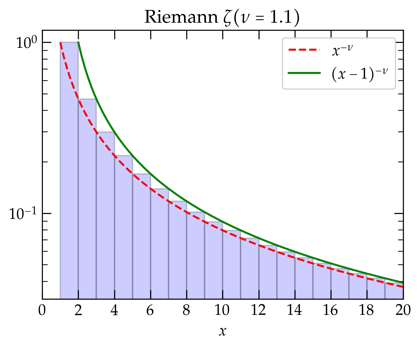
Figure 2 — The Riemann zeta function for \(\nu = 1.1\). The red and green curves clearly bound the area of the blue bars, which represents \(\zeta(1.1)\) (note the logarithmic vertical scale).
One place the Riemann zeta function pops up in physics is in the theory of blackbody radiation and the determination of the Stefan-Boltzmann constant, \(\sigma\), which relates the power per unit area radiated by an ideal blackbody at temperature \(T\): \begin{equation}\label{eq:Stefan-Boltzmann} p = \sigma T^4 \qquad\text{where}\qquad \sigma = \frac{6 \zeta(4) k_{\mathrm{B}}^4}{\pi^2 c^2 \hbar^3} = \frac{2 \pi^5 k_{\mathrm{B}}^4}{15 c^2 h^3} \approx 5.67 \times 10^{-8}\,\mathrm{W \cdot m^{-2} \cdot K^{-4}} \end{equation} In this expression, I have used that \(\displaystyle \zeta(4) = \frac{\pi^4}{90}\), which can be shown using contour integration.
If successive terms in a series alternate sign, and if the magnitude of the terms goes to zero as \(n\to\infty\), then the series converges. An infinite series is absolutely convergent if the sum of the absolute value of its terms converges. If the series converges, but it is not absolutely convergent, it is called conditionally convergent.
Properties of absolutely convergent series:
Note that none of these claims can be made for conditionally convergent series. As an illustration, consider the alternating harmonic series, \[ A = 1 - \frac12 + \frac13 - \frac14+\cdots = 1 - \left(\frac12 - \frac13\right) - \left(\frac14-\frac15\right) - \cdots \] The grouping seems clearly to show that \(A < 1\). We could also establish a lower bound by sliding the parentheses over one position: \[ A = \left(1 - \frac12\right) + \left(\frac13 - \frac14\right) + \left(\frac15 - \frac16\right) + \cdots \] which shows that \(A > \frac12\). As shown, for example, in Arfken, we could also group in the following way \begin{align} A &= \left(1 + \frac13 + \frac15 \right) - \left(\frac12\right) + \left( \frac17 + \frac19 + \frac{1}{11} + \frac{1}{13} + \frac{1}{15} \right) \notag \\ &\qquad - \left(\frac14\right) + \left( \frac{1}{17} + \cdots + \frac{1}{25}\right) - \left(\frac16 \right) + \cdots \label{eq:altharm} \end{align}
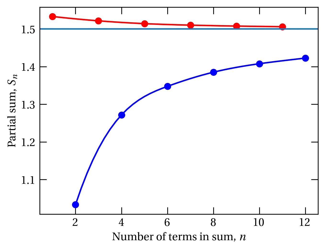
Figure 3 — Partial sums of the alternating harmonic series as grouped as illustrated in Eq. \eqref{eq:altharm}, which demonstrates convergence to 3/2.
Following is the matplotlib code to generate the figure:
from scipy.interpolate import make_interp_spline

highroad, lowroad = [],[]
nodd, neven = 1, 0
thesum = 1
while len(lowroad) < 6:
    while thesum < 1.5:
        nodd += 2
        thesum += 1/nodd
    highroad.append(thesum)
    neven += 2
    thesum -= 1/neven
    lowroad.append(thesum)

fig, ax = plt.subplots()
xhigh = np.arange(1, 2*len(highroad), 2)
xlow = np.arange(2, 2*len(lowroad)+1, 2)
sphigh = make_interp_spline(xhigh, highroad)
splow = make_interp_spline(xlow, lowroad)
ax.plot(xhigh, highroad, 'ro')
x = np.arange(1, 11.1, 0.25)
ax.plot(x, sphigh(x), 'r')
ax.plot(xlow, lowroad, 'bo')
x = np.arange(2, 12.1, 0.25)
ax.plot(x, splow(x), 'b')
ax.set_xlabel("Number of terms in sum, $n$")
ax.set_ylabel("Partial sum, $S_n$")
ax.axhline(1.5)
Next: Taylor Series