
You have encountered a few ordinary differential equations (ODEs) in chemistry, mechanics, engineering, and especially in Math 82. This page will serve as a quick reminder of some basic linear ODEs that are especially important in physics and some approaches to solving them. If you need a reminder about first-order differential equations, see here.
The most general second-order linear differential equation is \[ y^{\prime\prime} + P(x) y’ + Q(x) y = R(x) \] In this equation, \(x\) is the independent variable, \(y(x)\) is the dependent variable, and primes denote differentiation with respect to \(x\). The point \(x_0\) is called a regular point of the ODE if each of \(P(x)\) and \(Q(x)\) has a convergent power series expansion in the neighborhood of \(x_0\). A point for which this is not the case is called a singular point. A regular singular point is one for which both \((x-x_0)P(x)\) and \((x-x_0)^2 Q(x)\) have convergent power series in the neighborhood of \(x_0\). The method of Frobenius, which is outlined below, can be applied in the neighborhood of regular singular points; other singular points require more complicated techniques.
Some of the most important ODEs in physics include
| Equation | Form | Singular points |
|---|---|---|
| Damped SHO | $$y^{\prime\prime} + 2\beta y' + \omega_0^2 y = \frac{F(x)}{m}$$ | — |
| Equidimensional equation | $$y^{\prime\prime} + \frac1x y' + \frac{1}{x^2} y = 0$$ | — |
| Legendre’s equation | $$(1-x^2)y^{\prime\prime} - 2 x y' + \ell(\ell+1) y = 0$$ | $$\text{regular @ }x = \pm 1$$ |
| Bessel’s equation | $$x^2 y^{\prime\prime} + x y' + (x^2 - n^2) y = 0$$ | $$\text{regular @ }x = 0$$ |
| Generalized Laguerre equation | $$ x y^{\prime\prime} + (\alpha + 1 - x)y' + ny = 0$$ | $$\text{regular @ } x = 0$$ |
The solution to equidimensional equations may be obtained with the Ansatz (guess) \(y = x^p\), which reduces the differential equation to an algebraic equation.
Legendre’s equation arises when solving Laplace’s equation in spherical coordinates, such as when one seeks the eigenstates of the hydrogen atom.
Bessel’s equation describes the radial component of waves on a spherical membrane, or waves on a pond. Solutions oscillate with an amplitude that falls off (asymptotically) with distance \(x\) as \(1/\sqrt{x}\), consistent with energy conservation as the wave propagates outward.
The generalized Laguerre equation arises as the radial equation when solving for the eigenstates of the hydrogen atom.
One can learn a lot about the solutions to a second-order linear differential equation from the equation itself. As a simple example, consider the differential equation \[ y^{\prime\prime} + y = 0 \] This is a second-order linear differential equation with constant coefficients. Therefore, it has two linearly independent solutions; you already know that the solutions are \(\sin x\) and \(\cos x\).
But, suppose that you didn’t know that. Can we use the differential equation itself to derive the properties of the solutions?
With tongue in cheek (or malice of forethought), let us call the two solutions \(s(x)\) and \(c(x)\), and distinguish them by their properties at \(x = 0\). We will take \begin{align} s(0) &= 0 & \qquad s’(0) &= 1 \notag \\ c(0) &= 1 & \qquad c’(0) &= 0 \notag \end{align} and note that the general solution must take the form \[ y(x) = A c(x) + B s(x) \] Consider the derivative \(y'\). If we differentiate the original differential equation, we get \[ y^{\prime\prime\prime} + y’ = 0 \] Letting \(\eta = y'\), this equation may be written \[ \eta^{\prime\prime} + \eta = 0 \] which means that \(y' = \eta\) is also a solution to the original differential equation. Therefore, \(y'\) may be expressed as a linear combination of the eigenfunctions \(c(x)\) and \(s(x)\). So, for example, \[ s’(x) = \alpha c(x) + \beta s(x) \] At \(x = 0\), only \(c(x)\) is nonzero, so since we have assumed \(s'(0) = 1\), we must have \(\alpha = 1\), while \(\beta\) is as yet undetermined. Differentiating again, \[ s^{\prime\prime}(x) = c’(x) + \beta s’(x) = -s(x) \] At \(x = 0\), this implies \(0 = 0 + \beta \times 1\). Therefore, \(\beta = 0\) and we have determined that \[ s’(x) = c(x) \] The same reasoning starting with \(c'(x) = A c(x) + B s(x)\) and applying it at \(x = 0\) gives \[ c’(0) = 0 = A + 0 B \qquad\longrightarrow\qquad A = 0 \] Differentiating again gives \(c''(x) = -c(x)\), which at 0 yields \[ c^{\prime\prime}(0) = -c(0) = -1 = B s’(0) = B \qquad \longrightarrow\qquad c’(x) = -s(x) \] We can also establish the Pythagorean theorem! Note that at \(x = 0\), \(c(0)^2 + s(0)^2 = 1\). Now differentiate \(f = c^2(x) + s^2(x)\) with respect to \(x\): \[ f’ = 2c(x) c’(x) + 2 s(x) s’(x) = 2 c(x) [-s(x)] + 2 s(x) [c(x)] = 0 \] Since \(f'\) vanishes, \(f\) must be a constant and since it is 1 when \(x = 0\), it must be 1 for all \(x\).
Let us now consider a more general second-order linear differential equation, \[ y^{\prime\prime} = A(x) y’(x) + B(x) y(x) \] In a move reminiscent of the bilinear concomitant we encountered in developing orthogonality relations for the basis functions in a Fourier expansion, define the Wronskian of two functions as \(W(f,g) = f g' - g f'\). If each of \(f(x)\) and \(g(x)\) solves the differential equation, we can use the differential equation itself to simplify the derivative of the Wronskian, \[ \dv{W}{x} = f’ g’ + f g^{\prime\prime} - (g’ f’ + g f^{\prime\prime}) = f g^{\prime\prime} - g f^{\prime\prime} \] Now we take advantage of the fact that each function solves the differential equation: \begin{align} \dv{W}{x} &= f(x)[A(x) g’(x) + B(x)g(x)] - g(x)[A(x) f’(x) + B(x) f(x)] \notag \\ &= A(x) [f(x) g’(x) - g(x) f’(x)] = A(x) W(x) \notag \\ \frac{1}{W} \dd{W} &= A(x)\dd{x} \notag \\ \ln W &= \int A(x)\dd{x} \qquad\longrightarrow\qquad W(x) = c \exp\qty[\int A(x)\dd{x}] \label{eq:Abel} \end{align} Using this expression (known as Abel’s formula) and knowledge of one of the two solutions, we can generate a first-order equation to yield the other solution.
Consider the differential equation \begin{equation}\label{eq:BDP} x^2 y’’ + 2 x y’ - 2y = 0 \end{equation} for \(x > 0\). (a) Show that \(y_1(x) = x\) is a solution. (b) Use this solution and Abel’s formula to find the second solution, \(y_2(x)\).
The method of Frobenius is to way to solve differential equations that aren’t “too bad”—meaning that any singular points are regular. The method is quite simple. We assume a (Frobenius) series solution of the form \[ y(x) = \sum_{k=0}^{\infty} a_k x^{k+s} \] which is a generalization of a Taylor series that includes the possibility of negative or nonintegral powers, and substitute it into the differential equation. (\(s\) is an unknown constant.) We then perform appropriate index shifts to group all terms to the same power of \(x\). Since each power of \(x\) is a linearly independent function, the coefficient of For a homogeneous ODE, each of these must be zero.
To illustrate, let’s apply the method to Bessel’s equation, \begin{equation}\label{eq:Bessel} x^2 y^{\prime\prime} + x y’ + (x^2 - n^2) y = 0 \end{equation} See the section on Bessel’s equation for some background on why this equation arises in physical problems.
Substituting the Frobenius series into this equation gives \begin{align} x^2 \sum_{k=0}^\infty (k+s)(k+s-1)a_k x^{k+s-2} + x \sum_{k=0}^\infty (k+s) a_k x^{k+s-1} + \sum_{k=0}^\infty (x^2 - n^2) a_k x^{k+s} &= 0 \notag \\ \sum_{k=0}^\infty [(k+s)(k+s-1) + (k+s) - n^2 ] a_k x^{k+s} + \sum_{k=0}^\infty a_k x^{k+s+2} &= 0 \notag \\ x^s \qty{\sum_{l=0}^\infty [(s+l)^2 - n^2] a_l x^l + \sum_{l=2}^\infty a_{l-2} x^l } &= 0 \label{eq:Frob} \end{align} There is only one term in the sums with \(l = 0\). Although we could choose \(a_0 = 0\), that would just shift the start of the series (effectively shifting \(s\)). So, if \(a_0 \ne 0\), then we must have for \(l = 0\) that \[ s^2 = n^2 \qquad\longrightarrow\qquad s = \pm n \] This equation is called the indicial equation. Taking \(a_0 = 1\), we next have to consider the case when \(l = 1\) (assuming that \(s = \pm n\)). From Eq. \eqref{eq:Frob}, we have \[ [(s+1)^2 - n^2]a_1 = 0 \] which requires that \(a_1 = 0\). So, all the odd coefficients vanish, and the next required relationship between coefficients happens for \(l = 2\). Combining the series for \(l \ge 2\), we have \[ a_0 + \sum_{l=2}^\infty \qty[(l^2 \pm 2 n l)a_l + a_{l-2} ] x^l \] Therefore, \[ a_l = - \frac{a_{l-2}}{l(l \pm 2n)} \] Let’s use this recursion relation to solve for \(J_0(x)\), the zeroth-order Bessel function of the first kind for \(n = 0\). \begin{align} a_0 &= 1 \notag \\ a_2 &= - \frac{a_0}{2^2} \notag \\ a_4 &= - \frac{a_2}{4^2} = \frac{1}{(2 \cdot 4)^2} \notag \\ a_{2k} &= (-1)^k \frac{1}{2^{2k}} \qty(\frac{1}{k!})^2 \notag \end{align} which we can combine to form \[ J_0(x) = 1 - \qty(\frac{x}{2})^2 + \frac{1}{(2!)^2} \qty(\frac{x}{2})^4 - \frac{1}{(3!)^2} \qty(\frac{x}{2})^6 + \cdots \]
What does this look like?
def myJ0(x, n_max=16):
    j0, y = 1, (x/2)**2
    a, yn = 1, 1
    for n in range(1, n_max+1):
        a /= -(n*n)
        yn *= y
        j0 += a * yn
    return j0

fig, ax = plt.subplots()
x = np.pi * np.linspace(0, 3, 101)
y = myJ0(x)
ax.plot(x, y)

# Now let's add the scipy version
from scipy.special import jv
j0 = jv(0, x)
ax.plot(x, j0, '.')
ax.set_xlabel("$x$")
ax.set_ylabel(r"$J_0(x)$");
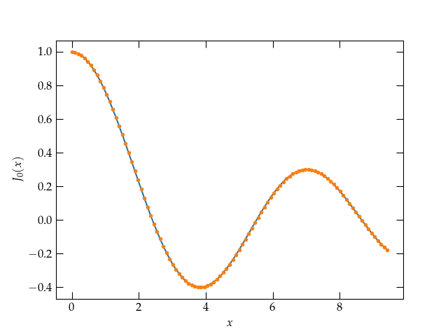
Figure 1 — The behavior of \(J_0(x)\) for small \(x\) computed via myJ0 (smooth curve) and scipy.special.jv (dots).
You can readily see the fine agreement between the truncated series and the scipy version of \(J_0(x)\).
Next: Numerical Approaches