
NumPy (“num-pie”) is a Python library of optimized routines for computing with arrays. Compared to writing loops over nested lists, as in normal Python syntax, operating with NumPy routines on NumPy arrays greatly accelerates operations and uses more readable syntax.
The standard way to access the routines of NumPy in a Python program is with an import statement of the form
import numpy as np
A basic numerical type in NumPy is the np.ndarray, which can represent an array of arbitrary numbers of dimensions. You can create an array from basic Python types such as lists and tuples using np.array(list_or_tuple). For example
a = np.array([[1, 2, 3], [4, 5, 6]])
generates the \(2\times 3\) array
array([[1, 2, 3],
       [4, 5, 6]])
Besides listing all elements of a NumPy array, you can use a number of convenience functions to generate them:
np.arange(start, end, dx) generates a one-dimensional array of values (start, start + dx, start + 2 * dx, …, start + n * dx) where the final value satisfies start + n * dx < end. For instance, np.arange(1, 4, 1) produces array([1, 2, 3]). That is, the final value in the array is smaller than the second argument.np.linspace(start, end, n) generates a one-dimensional array of values that divides [start, end] into \(n-1\) equal intervals, so that np.linspace(1, 4, 4) produces array([1, 2, 3, 4]). That is, linspace includes the end points, whereas arange does not include its end point.np.zeros((nrows, ncols)) generates an array with nrows and ncols filled with zeros. You can include any number of dimensions in the tuple that specifies the size of the array.np.zeros(nelements, dtype=np.int8)np.ones((nrows, ncols)) generates an array of ones.A is already an array (or might be some other iterable), use np.asarray(A), rather than np.array(A). Why? Because np.asarray(A) does not create a copy if it doesn’t need to, whereas np.array(A) creates a copy of A regardless.Suppose that you want to multiply each element in a list by 3.2. In standard Python, you could write a list comprehension of the form
b = [x * 3.2 for x in mylist]
for a list stored in mylist. If, instead, you use a NumPy array, you can simplify the notation to eliminate explicit loops:
b = np.asarray(mylist) * 3.2
This notation also works for multiplying (or performing similar arithmetic operations) on all elements of a NumPy array of arbitrary dimensions.
All of the standard functions have NumPy versions that “broadcast” in this way over the elements of the array that they are passed. So, the following code computes a comb of equally spaced \(x\) values and computes the corresponding sine values and then uses matplotlib to plot the result:
import numpy as np
import matplotlib.pyplot as plt

t = np.linspace(0, 1, 51)      # create an array of equally spaced t values
y = np.sin(x * 2 * np.pi)      # compute sine values via broadcasting
z = np.cos(x * 2 * np.pi)      # compute cosine values via broadcasting
fig, ax = plt.subplots()       # start a matplotlib plot
ax.plot(x, y, 'b.', label=r'$\sin(2\pi t)$') # 'b.' means blue dots
ax.plot(x, z, 'ro', label=r'$\cos(2\pi t)$') # 'ro' means red circles
ax.set_xlabel('$t$')           # dollar signs turn on LaTeX; t is italicized
ax.legend();                   # use labels to create a legend
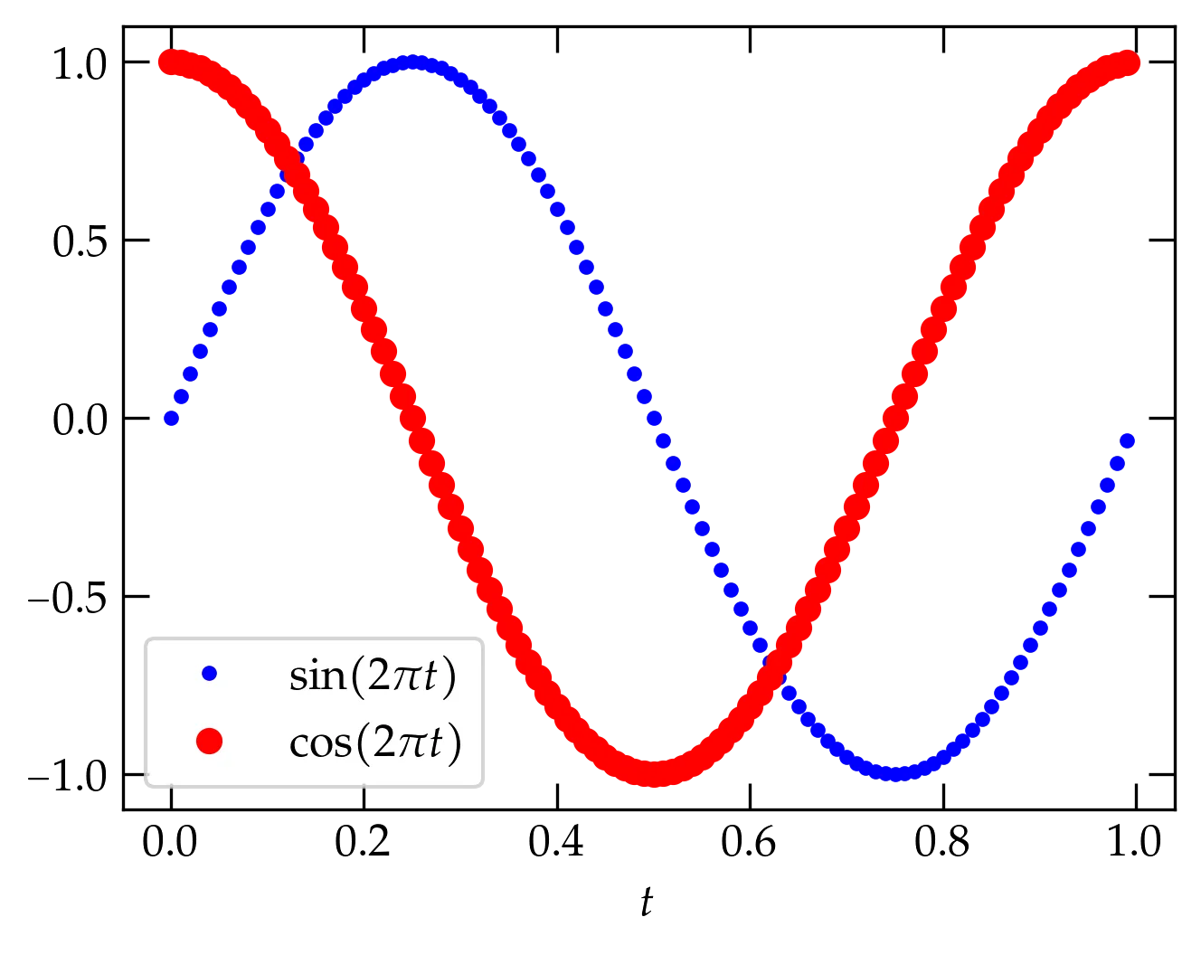
Figure 1 — Plot of \(\sin(2\pi t)\) and \(\cos(2\pi t)\) on the interval \([0, 1]\). Note that my preferences set usetex=True automatically, so that text between dollar signs is fed through TeX. If you don’t see proper rendering, try including the optional keyword argument usetex=True in the two set_label commands.
Functions that “broadcast” across the elements of an array are called universal functions. You can read more about NumPy’s universal functions in the official documentation. They include all the standard trigonometric, exponential, and hyperbolic functions, degree-radian conversions, rounding, etc. Some “unusual” ones you might find handy:
square(x) computes the square of all elements of xcbrt(x) computes the cube root of all elements of xarctan2(y, x) computes the arctangent of (x,y) points, in radians, making sure to get the quadrant correctdegrees(x) converts values in x from radians to degrees; rad2deg(x) does the same thingisnan(x) returns a boolean array of True values if x is not a number and False otherwisefloor(x) returns the greatest integer less than each value of x; see also round(x) and trunc(x)Sometimes you want to operate row-wise or column-wise on a two-dimensional array. Consider the following example:
from numpy.random import default_rng
rng = default_rng()                     # initialize a random number generator
m = np.around(rng.uniform(-5., 5., size=(2, 3)), 1)
m                                       # make a row of random numbers in [-5.0, 5.0) with 2 rows and 3 columns
array([[-1.5,  4.8, -0.7],              # but round to one digit after the decimal point
        [ 3.4, -4.8,  2.7]])

m.shape                                 # describe the size of m
(2, 3)

m.max()                                 # what is the single largest value in the array?
4.8

m.max(axis=0)                           # what is the largest value in any row
array([3.4, 4.8, 2.7])                  # three answers, one for each column

m.max(axis=1)                           # what is the largest value in any column
array([4.8, 3.4])                       # two answers, one for each row
This approach is not limited to two-dimensional arrays:
m3 = np.around(rng.uniform(-10., 10., size=(2,3,4)), 1)
m3
array([[[ 6.1,  0.2, -2.8,  3.8],
        [ 8.1,  4.5, -3.1, -4.1],
        [ 8.2,  0.1, -0.8, -5.6]],

        [[ 9.3, -5.6, -6.2, -5.6],
        [ 1.6,  0.2,  4.6, -8.5],
        [ 5.8, -1.9,  1.2,  6. ]]])
m3.max()            # the maximum of all elements
9.3
m3.max(axis=0)      # the maximum in each row
array([[ 9.3,  0.2, -2.8,  3.8],
        [ 8.1,  4.5,  4.6, -4.1],
        [ 8.2,  0.1,  1.2,  6. ]])
m3.max(axis=1)      # the maximum in each column
array([[ 8.2,  4.5, -0.8,  3.8],
        [ 9.3,  0.2,  4.6,  6. ]])
m3.max(axis=2)      # the maximum in each chunk
array([[6.1, 8.1, 8.2],
        [9.3, 4.6, 6. ]])
m3.max(axis=(0,1))  # the maximum in each (row, col) portion
array([9.3, 4.5, 4.6, 6. ])
In short, functions such as sum, max, min, etc., operate by default on all elements of multidimensional arrays, but can also be specialized to work along various axes (directions) of the array.
Like lists and tuples, NumPy arrays understand slices. To extract the first column (column 0) from m, use m[:,0]:
m[:,0]
array([-1.5,  3.4])

m[1,:]
array([ 3.4, -4.8,  2.7])
Note that the “bare” colon means all; you can use start:stop or start:stop:stride syntax, as well.
p = np.array(range(12))
array([ 0,  1,  2,  3,  4,  5,  6,  7,  8,  9, 10, 11])

p[0:10:2]
array([0, 2, 4, 6, 8])
Sometimes you want to know not just what the largest value is but where it is in the array.
np.argmax(m3)                           # where is the largest element
12                                      # 9.3 is at offset 12 (the 13th element)

np.argmax(m3, axis=0)
array([[1, 0, 0, 0],
        [0, 0, 1, 0],
        [0, 0, 1, 1]])

np.sort(m3)                             # sort over the last index of the array
array([[[-2.8,  0.2,  3.8,  6.1],
        [-4.1, -3.1,  4.5,  8.1],
        [-5.6, -0.8,  0.1,  8.2]],

        [[-6.2, -5.6, -5.6,  9.3],
        [-8.5,  0.2,  1.6,  4.6],
        [-1.9,  1.2,  5.8,  6. ]]])
You can also sort over other axes.
sum(x) computes the sum of all elements, but you can also use axis= to adjust what is summedproduct(x) multiplies all elementscumsum(x) (cumulative sum) returns an array in which the nth value is the sum of all entries up to and including the nth valuecumprod(x) (cumulative product) like cumsum but multiplies all prior elements togethernansum(x) compute the sum of all values in x that are not NaNs (not a numbers)