
We saw on the page describing how to solve second-order ODEs numerically that the trick is to rewrite them as systems of coupled first-order ODEs and use a solver such as scipy.integrate.solve_ivp to perform the integration while simultaneously bounding the error. In practice, it may take some fiddling with the integration method and the error tolerances rtol and atol to obtain acceptable results.
As Prof. Tamayo can readily explain, however, the Runge-Kutta solvers available in solve_ivp have a property that makes them less than ideal for integrating equations of motion over very extended periods. To illustrate, let’s repeat our simulation of the simple harmonic oscillator and focus not so much on \(x(t)\) but on the sum of kinetic and potential energy in the computed solution. The system is clearly conservative, so we should expect the energy to remain constant. Let’s see.
def SHOderiv(t, Y, k, m):
    x, v = Y
    return (v, -k * x / m)

k, m = 1, 1
s = solve_ivp(SHOderiv, (0, 100), (np.sqrt(2),0), t_eval=np.arange(0, 100, 0.1),
              rtol=1e-6, atol=1e-6, method='RK45', args=(k, m))
# Compute the oscillator energy
x = s.y[0,:]
v = s.y[1,:]
E = 0.5 * (k * x**2 + m * v**2)
fig, ax = plt.subplots()
ax.plot(s.t, E);
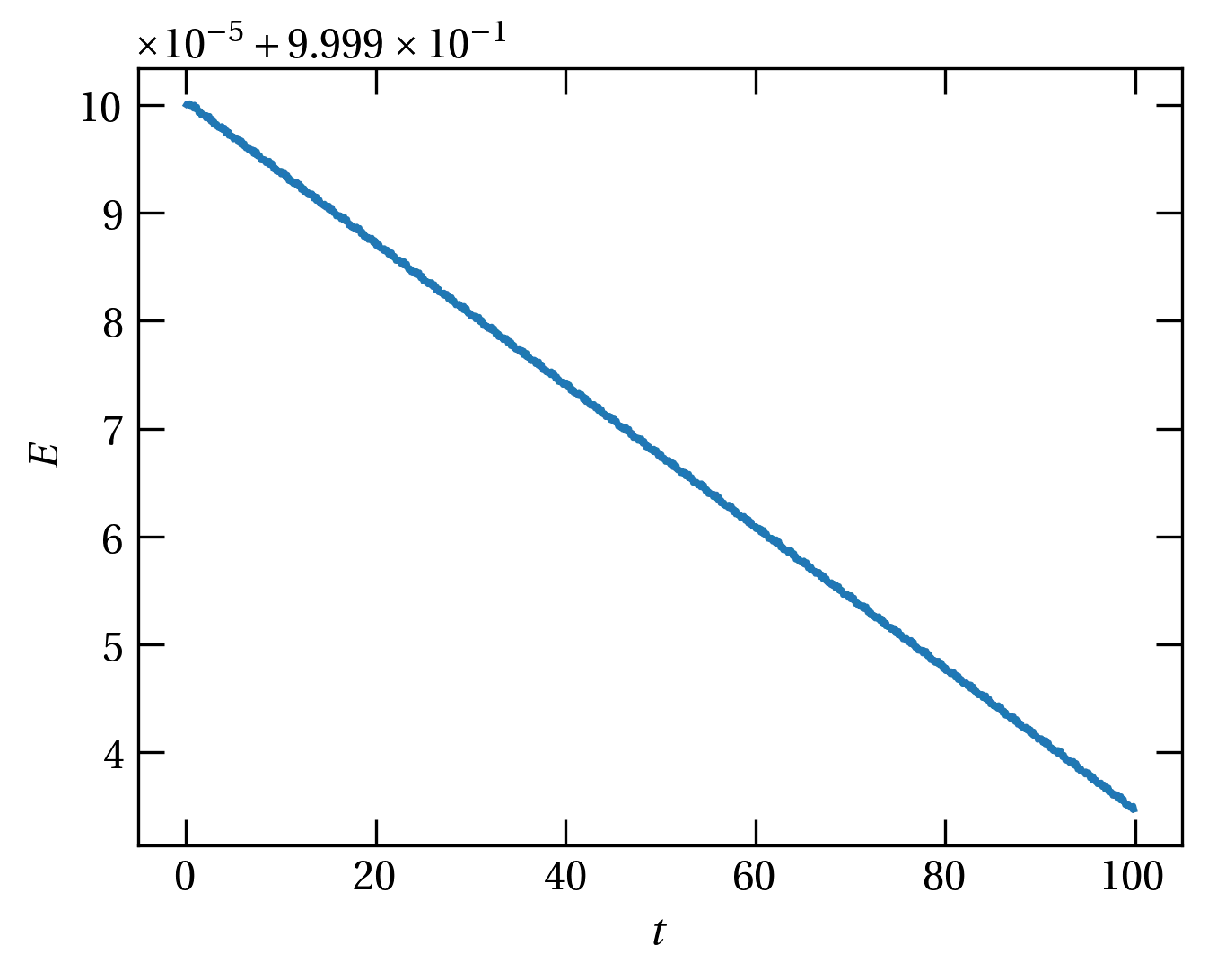
Figure 1 — The sum of kinetic and potential energy in a numerical solution of the SHO equation of motion. Tightening the tolerances reduces the scale of the error but not the general downward trend.
In Runge-Kutta integrators, all dependent variables are updated in parallel. That is, at each (sub) time step, all derivatives are computed and used to advance each dependent variable. By contrast, in the leapfrog approach,
The method is called leapfrog, because we alternately update the position and the velocity, using always the most recent values of \((x,v)\) for the updates.
More generally, a symplectic integrator subdivides a time step \(\Delta t\) into \(k\) parts, and for each part, updates first the velocity and then the position using the equations \begin{align} v_i &= v_{i-1} + (\Delta t) c_i a(x_{i-1}) \label{eq:vupdate} \\ x_i &= x_{i-1} + (\Delta t) d_i v_i \label{eq:xupdate} \end{align} The leapfrog method uses \(c_i = (\frac12, \frac12)\) and \(d_i = (1, 0)\) and is second order (\(k=2\)). Higher-order methods are possible, too. A third-order integrator uses \(c_i = (\frac{7}{24}, \frac34, -\frac{1}{24})\) and \(d_i = (\frac23, -\frac23, 1)\), and a fourth-order one uses (\(q \equiv 2^{1/3}\)) \begin{align} c_1 = c_4 &= \frac{1}{2(2-q)} \\ c_2 = c_3 &= \frac{1-q}{2(2-q)} \\ d_1 = d_3 &= \frac{1}{2-q} \\ d_2 &= - \frac{q}{2-q} \\ d_4 &= 0 \end{align}
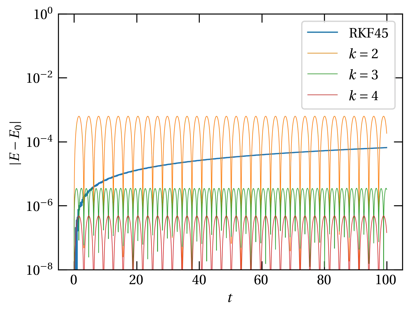
Figure 2 — The degree of energy nonconservation, \(|E - E_0|\), as a function of time for the simple harmonic oscillator integrated with the RKF45 method by solve_ivp and by symplectic integrators of order \(k\). The RKF45 routine uses an adaptive step size to bound the error, whereas the symplectic integrators all used a step size \(\Delta t = 0.05\). Unlike the Runge-Kutta method, whose energy errors grow quasi-monotonically, the energy errors of the symplectic integrators oscillate.
I’m going to use the SHO as the example. The equation of motion is \begin{equation}\label{eq:SHO} \ddot{x} + \omega^2 x = 0 \end{equation} We now break it apart into two coupled first-order differential equations: \begin{align} \dv{x}{t} &= v \\ \dv{v}{t} &= -\omega^2 x \end{align} and use the following simple Euler integration scheme for a time step \(\Delta t\): \begin{align} v_{n+1} &= v_n + (-\omega^2 x_n) \Delta t \label{eq:vn1}\\ x_{n+1} &= x_n + v_{n+1} \Delta t \label{eq:xn1} \end{align}
We will now look for a matrix \(\mat{M}\) such that \[ \begin{pmatrix} x_{n+1} \\ v_{n+1} \end{pmatrix} = \mat{M} \begin{pmatrix} x_{n} \\ v_{n} \end{pmatrix} \] which we will be able to use to characterize the stability of the integrator.
To find \(\mat{M}\), we will reorganize Eqs. \eqref{eq:vn1} and \eqref{eq:xn1} to put all values at interval \(n+1\) on the left and the rest on the right: \begin{align} x_{n+1} - v_{n+1} \Delta t &= x_n \notag \\ v_{n+1} &= v_n - \omega^2 x_n \Delta t \notag \end{align} or \[ \underbrace{\begin{pmatrix} 1 & -\Delta t \\ 0 & 1 \end{pmatrix}}_{\mat{m}} \begin{pmatrix} x_{n+1} \\ v_{n+1} \end{pmatrix} = \begin{pmatrix} 1 & 0 \\ -\omega^2 \Delta t & 1 \end{pmatrix} \begin{pmatrix} x_n \\ v_n \end{pmatrix} \] Noting that \[ \mat{m}^{-1} = \begin{pmatrix} 1 & \Delta t \\ 0 & 1 \end{pmatrix} \] and multiplying from the left we get \begin{equation}\label{eq:M} \begin{pmatrix} x_{n+1} \\ v_{n+1} \end{pmatrix} = \begin{pmatrix} 1 & \Delta t \\ 0 & 1 \end{pmatrix} \begin{pmatrix} 1 & 0 \\ -\omega^2 \Delta t & 1 \end{pmatrix} \begin{pmatrix} x_n \\ v_n \end{pmatrix} = \underbrace{\begin{pmatrix} 1 - (\omega\Delta t)^2 & \Delta t \\ -\omega^2 \Delta t & 1 \end{pmatrix}}_{\mat{M}} \begin{pmatrix} x_n \\ v_n \end{pmatrix} \end{equation}
The matrix \(\mat{M}\) is called the propagator: it tells us how to propagate the state vector at time \(n\) to the state vector at time \(n+1\). By induction, \begin{equation}\label{eq:propagation} \begin{pmatrix} x_{n} \\ v_{n} \end{pmatrix} = \mat{M}^n \begin{pmatrix} x_{0} \\ v_{0} \end{pmatrix} \end{equation}
Knowing that energy of the SHO is a conserved quantity, intuitively we must have that successive applications of \(\mat{M}\) do not cause the state vector either grow or shrink, or the energy will grow or shrink with time.
To make that more precise, we could take as our initial state \[ \begin{pmatrix} x_0 \\ v_0 \end{pmatrix} = A_0 \begin{pmatrix} e^{-i\omega t} \\ -i\omega e^{-i\omega t} \end{pmatrix} \] where \(A_0\) is the initial amplitude and I have explicitly used an exact solution to the differential equation. Now we propagate to the next step: \[ \begin{pmatrix} x_1 \\ v_1 \end{pmatrix} = A_1 \begin{pmatrix} e^{-i\omega t} \\ -i\omega e^{-i\omega t} \end{pmatrix} = A_0 \mat{M} \begin{pmatrix} e^{-i\omega t} \\ -i\omega e^{-i\omega t} \end{pmatrix} \] or dividing out \(e^{-i\omega t}\), \[ A_1 \begin{pmatrix} 1 \\ -i\omega \end{pmatrix} = A_0 \mat{M} \begin{pmatrix} 1 \\ -i\omega \end{pmatrix} \] For stability, we require that \(|A_1| = |A_0|\); the amplitude should remain constant.
The matrix \(\mat{M}\) is not diagonal in the \((x_n, v_n)\) basis. Suppose we find a matrix \(\mat{S}\) such that \begin{equation}\label{eq:similarity} \mat{S}^{-1}\widetilde{\mat{M}}\mat{S} = \mat{M} \end{equation} where \(\widetilde{\mat{M}}\) is diagonal. Equation \eqref{eq:similarity} is called a similarity transformation. It is a change of basis that yields a diagonal representation of matrix \(\mat{M}\). Since \(\widetilde{\mat{M}}\) is diagonal, we can write \begin{equation}\label{eq:mtilde} \widetilde{\mat{M}} = \begin{pmatrix} \gamma_+ & 0 \\ 0 & \gamma_- \end{pmatrix} \end{equation} Then \[ \mat{M}^n = (\mat{S}^{-1}\widetilde{\mat{M}}\mat{S}) (\mat{S}^{-1}\widetilde{\mat{M}}\mat{S})\cdots (\mat{S}^{-1}\widetilde{\mat{M}}\mat{S}) = \mat{S}^{-1}\widetilde{\mat{M}}^n\mat{S} = \mat{S}^{-1}\begin{pmatrix} \gamma_+^n & 0 \\ 0 & \gamma_-^n \end{pmatrix} \mat{S} \] Unless \(|\gamma_{\pm}| = 1\), the solution in the diagonal basis will grow or shrink in magnitude over time, which is inconsistent with energy conservation.
To solve for the eigenvalues \(\gamma_{\pm}\), we calculate \[ \det \begin{pmatrix} 1 - \omega^2 (\Delta t)^2 - \gamma & \Delta t \\ -\omega^2 \Delta t & 1 - \gamma \end{pmatrix} = 0 \] which simplifies to \begin{equation}\label{eq:gain} \gamma^2 + \gamma[\omega^2 (\Delta t)^2 - 2] + 1 = 0 \end{equation} Let \(\theta \equiv \omega \Delta t\); it represents the angle through which the phase of the oscillator moves in the interval \(\Delta t\). Then \begin{align} \gamma &= \frac{2 - \theta^2 \pm \sqrt{4 - 4\theta^2 + \theta^4 - 4}}{2} \notag \\ &= 1 - \frac{\theta^2}{2} \pm \theta \sqrt{\frac{\theta^2}{4}-1} \notag \\ &= 1 - \frac{\theta^2}{2} \pm i\theta \sqrt{1-\frac{\theta^2}{4}} \end{align} For \(\theta < 2\), the radical is real and \(\gamma\) is complex. It’s magnitude is \[ |\gamma|^2 = \left(1 - \theta^2 + \frac{\theta^4}{4}\right) + \theta^2 \left(1 - \frac{\theta^2}{4}\right) = 1 \] Wow. This means that for \(\theta < 2\), the eigenvalues (gain) have magnitude 1, which means that the solution neither grows nor shrinks over time.
Next: Quantum SHO