
Newton’s equations of motion (in one dimension) are typically second-order differential equations of the form \(\displaystyle m \dv[2]{x}{t} = F(x, v, t)\) where \(v = \dv{x}{t}\) and \(F\) is some function of the position, velocity, and time. To get our feet wet on how to solve such equations numerically, let’s start with a simpler situation in which the acceleration is proportional to the velocity, \(m \dot{v} = f(v)\) where the dot indicates differentiation with respect to time and \(f\) is a known function that depends only on the velocity \(v\). This form could describe, for example, a ball bearing moving through a viscous fluid.
One way to visualize this equation is to show the slope \(\dv{v}{t} = f(v)/m\) as a function of \(t\) and \(v\) in a slope field. We start at a particular value of \(v\) at \(t = 0\) and follow the local value of slope to determine how the value of \(v\) should change in the next small interval of time. This takes us to a new value of \(v\), from which we can determine a new value of slope and then a new value of \(v\), etc. The result is illustrated by the light red line in the figure below.
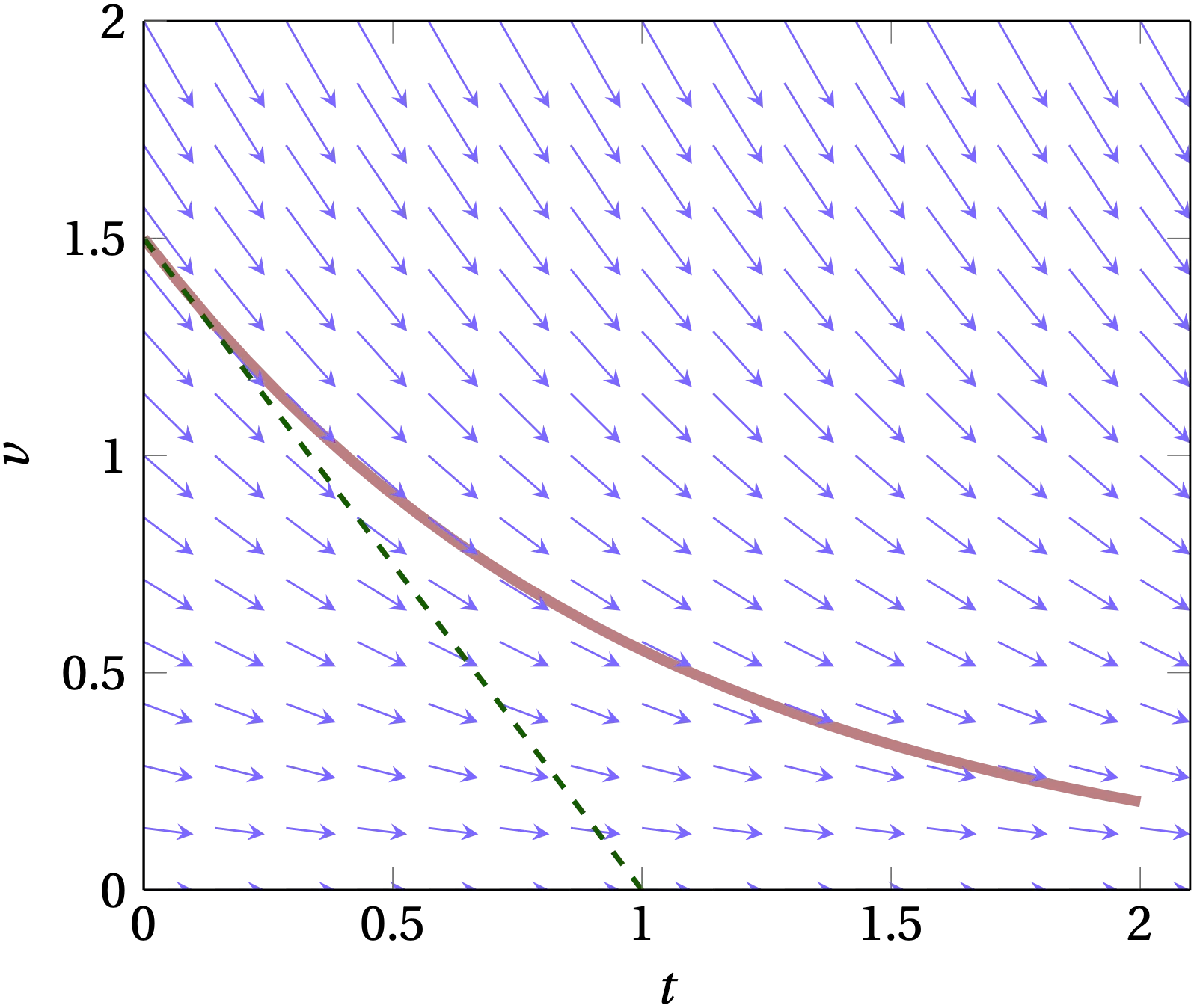
Figure 1 — The arrows show the derivative \(\dot{v}\); the red curve shows an example solution to the first-order equation, while the dashed green line shows the continuation of the slope from its value at \(t = 0\).
Let us take the first-order differential equation above and simplify it by moving the mass to the right-hand side, \(\dv{v}{t} = \frac{1}{m} f(v)\) which we can also write suggestively as \begin{equation} \dd{v} = \frac{f(v)}{m} \dd{t} \label{eq:DE} \end{equation} Conceptually, this equation says that if we know \(v(t)\) at some moment of time \(t\), we know how \(v\) will change in the next infinitesimal increment of time \(\dd{t}\); the rate of that change is just given by \(f(v)/m\). However, this expression is only true in the limit that \(\dd{t}\) is infinitesimal (infinitely tiny), which means that we would need to apply this rule an infinite number of times to cover even a modest (finite) time interval.
We would much rather take time steps larger than “infinitely small,” so that we can cover a finite interval of time in a finite number of steps. In that case,
\begin{equation} \delta v \approx \frac{f(v)}{m} \delta t \end{equation}
where \(\delta t\) is now a small but finite interval of time. This equation embodies Euler’s method of approximating the solution of a differential equation: it pretends that the derivative doesn’t change over the finite time interval \(\delta t\), which is only really true if \(f(v)\) is a constant. (I am going to reserve \(\Delta t\) to represent an extended interval of time, which we might break up into a number of smaller steps \(\delta t\) to which we apply the above equation.)
To see how successfully Euler’s method works, let’s consider a situation where the damping force on a particle of mass \(m\) is proportional to the particle’s velocity,
\begin{equation} f(v) = -b v \label{eq:damping} \end{equation} where \(b\) is a constant whose dimensions in SI units would be newton-seconds per meter. This viscous damping force is definitely not independent of the particle’s velocity; as the particle slows down, the damping force retarding its further motion diminishes. Therefore, we should expect that using Euler’s method will tend to be increasingly inaccurate the larger we make the time steps \(\Delta t\). Let’s test that hypothesis using in a Jupyter notebook. First, we’ll use nothing but the straight Python you have already learned. Then we’ll introduce some refinements.
At the top of the notebook, enter
%matplotlib widget
import numpy as np
import matplotlib.pyplot as plt
The first line enables graphics output by matplotlib to be embedded in the
notebook; the other two load the numpy and matplotlib modules. If you are using the older Jupyter Notebook, change widget to notebook in the first line.
b = 1      # the damping coefficient (you can change this value)
m = 1      # the particle mass (you can change this, too)
v0 = 5     # the initial velocity
dt = 0.1   # the time step (you can also change this, if you like)
v = [v0,]  # initialize an array of velocities
t = [0, ]  # and an array of times
while t[-1] < 1:
    dv = -b / m * v[-1] * dt  # compute the change in velocity, assumed constant over time interval
    v.append(v[-1] + dv)      # append the new velocity to the growing array of velocities
    t.append(t[-1] + dt)      # and append the new time

# Solving exactly gives the equation v(t) = v0 * exp(-b/m t)
# Let's plot the comparison between the Euler’s-method solution and the true function

fig, ax = plt.subplots()   # create a plot
ax.plot(t, v, 'ro', label='Euler')
ax.plot(t, v0 * np.exp(-b/m * np.array(t)), 'b-', label='true')
ax.set_xlabel('$t$')
ax.set_ylabel('$v$')
ax.legend();
The results are shown in Fig. 2, which indicates that the values calculated using Euler’s method lie below the true solution to the differential equation, which is \(v(t) = v_0 \exp(-\frac{b}{m} t)\).
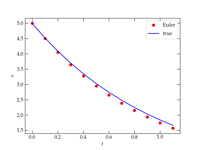
Figure 2 — Euler’s method (red dots) compared to the true solution to the differential equation.
Can you explain why the dots lie below the line?
One way to explore how (in)accurate Euler’s method is would be to plot the difference between its predictions and the correct answer. We would expect these differences to grow over time; the more steps we take, the farther away from the correct solution we will stray. It will be convenient to write first a little function to “run” Euler’s method. It will take a list of time values and the starting velocity and then calculate all the remaining velocities.
def Euler(tvals, v0, b=1, m=1):
    """Starting at v0 at the first entry in tvals, use Euler's
    method to integrate the first-order differential equation to
    find v at each of the remaining tvals.
    """
    v = [v0,] # initialize the output array
    for n in range(1, len(tvals)):
        dt = tvals[n] - tvals[n-1] # in case the time steps aren't even
        dv = -b * v[-1] * dt / m
        v.append(v[-1] + dv)
    return np.array(v)
We can now use this routine to explore the errors.
def EulerError(nsteps:list, b=1, m=1, v0=5):
    """Prepare a graph showing errors accumulated by using Euler's
    method to integrate a first-order differential equation.
    """
    assert isinstance(nsteps, (tuple, list, np.ndarray)), "Pass in a list of positive integers"
    fig, axes = plt.subplots(1, 2, figsize=(8, 4))  # create an empty plot
    ax1, ax2 = axes
    ax1.set_xlabel('$$t$$')
    ax1.set_ylabel('$$v$$')
    ax2.set_xlabel('$$t$$')
    ax2.set_ylabel('Error')
    for n in nsteps:
        tvals = np.linspace(0, 1.0, n+1) # linspace divides the span between the arguments into n equal steps
        vvals = Euler(tvals, v0, b, m)
        ax1.plot(tvals, vvals, '.-', label=str(n))
        ax2.plot(tvals, np.abs(vvals - v0 * np.exp(-tvals * b/m)), '.-', label=str(n))
    ax1.legend()

EulerError([2, 4, 8, 16]) # Cover the [0,1] range in 2, 4, 8, and 16 steps
The results for crossing the 1-second time interval in 2, 4, 8, and 16 steps are shown in Fig. 3. Clearly, the smaller the steps we take, the more accurate the numerical approximation is. We could quantify
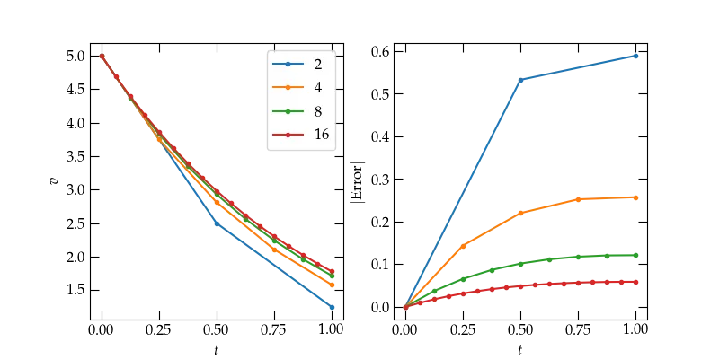
Figure 3 — Euler’s method solution (left) and absolute error (right) for different numbers of steps. Clearly, taking smaller steps leads to smaller final error. But how efficiently?
Prepare a plot that shows how the error after 1 second depends on the size of
the time step \(\dd{t} = (1~\mathrm{s}) / n\), where \(n\) is the number of equal steps
used to subdivide the 1-second interval. You can use the Euler function above
to do much of the computing, along with np.linspace to produce the time
values.
Hints:
ax.plot(...), use ax.loglog(...).Your results from the previous exercise might persuade you that the secret to an accurate numerical solution is just to take lots of tiny steps—a sort of “brute force” approach.
The upshot of our investigation of Euler’s method is that it has two salient properties, one good, and one bad:
Fortunately, there are much better ways. I won’t drag you through all the interesting applications of Taylor’s theorem which can be used to explore how the errors depend on step size of various methods, but I can offer a hint of the basic idea. Many of the methods are founded on the insight that it is bad strategy to base the behavior over the entire step on the derivative we calculate at the beginning of the step. It would be smarter to use the initial derivative to make a tentative first step, say, half-way across the full step \(\delta t\), then see what the derivative looks like there. We could then use that value of the derivative to try another half-way step, which would land us in a slightly different spot and with a slightly different slope. Somehow, we then combine all this information to take the full step. In a nutshell, this is the recipe in the celebrated Runge-Kutta method, which is fourth-order in \(\delta t\). (It was developed around 1900 by the German mathematicians Carle Runge and Wilhelm Kutta.) That is, if you take twice as many steps to cross a given time range, the error should drop by a factor of 16! Now we’re talking!
Many years later, some folks realized that it would be nifty if the same
intermediate points we calculate while working up the courage to step across
\(\delta t\) could be used for two methods of different order. The standard
Runge-Kutta-Fehlberg 4th-5th order does this, using the difference between the
two methods to estimate the error of the step. The RK45 method is the
default method used by the scipy function solve_ivp which we will use instead
of Euler’s method. This method is a real workhorse and should suffice for almost
all of our work. (However, see Prof. Tamayo on alternative strategies which do a better job of conserving energy in propagating equations of motion.) First, we need to import the routine.
from scipy.integrate import solve_ivp
To use this routine, let me remind you of the problem we’re trying to solve. In a nutshell, it is that we have a function that computes the derivative,
\begin{equation}\label{eq:theDE} \frac{dy}{dt} = f(t, y) \end{equation}
and we are trying to solve for \(y(t)\) assuming that we know the value of \(y(t_0) = y_0\). In the case of the pearl sliding through the viscous fluid, \(y\) represented the pearl’s velocity \(v\) and the function \(f(t, y)\) took the form \(f(t, y) = - y \times b / m\) As in this case, we commonly need to pass the function \(f\) additional parameters, such as \(b\) and \(m\), so we will define the derivative function as follows:
def myderiv(t, v, b, m):
    """Given the current value of v and t, and the parameters
    b (damping) and m (mass), compute and return the derivative."""
    return -v * b / m
Now, we can use the function solve_ivp to integrate Eq. \eqref{eq:theDE} from a starting
value of \(y\) at \(t = 0\). At a minimum, we need to supply the name of the
function that computes the derivative, the time interval over which to
integrate, and the initial value \(y_0\). If our derivative function takes
additional parameters (as ours does), we need to supply the extra parameters in
a tuple as the args keyword argument, as shown below.
b, m = 1, 1
res = solve_ivp(myderiv, [0, 1], [5.0], t_eval=np.linspace(0, 1, 11), args=(b, m))
res

    message: 'The solver successfully reached the end of the integration interval.'
        nfev: 14
        njev: 0
        nlu: 0
        sol: None
    status: 0
    success: True
        t: array([0. , 0.1, 0.2, 0.3, 0.4, 0.5, 0.6, 0.7, 0.8, 0.9, 1. ])
    t_events: None
        y: array([[5.        , 4.52418709, 4.09326263, 3.70297271, 3.34989891,
        3.03077272, 2.74247553, 2.48203859, 2.24664309, 2.03362008,
        1.84045052]])
    y_events: None
As you can see from res, the call to solve_ivp completed successfully; it
required 14 evaluations of the function myderiv; and returned the time values at
which we requested output by passing the keyword parameter t_eval with a list
(array) of time values, along with the computed values of 𝑦. We can get a sense
of the errors that this “marvelous” routine computed for us with the following:
errors = res.y[0,:] - 5.0 * np.exp(-res.t * b / m)
fig, ax = plt.subplots()
ax.plot(res.t, errors, 'ro');
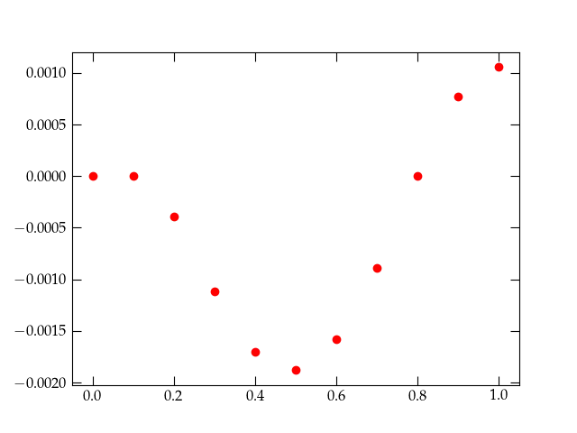
Figure 4 — The errors from a call to solve_ivp using default parameters. Do you think they are acceptable?
solve_ivpYou probably find that the errors reported in Fig. 4 are a bit
large for your taste. It depends on the application. If it took a long time to
compute the derivative function myderiv, we might be satisfied with these
results. But, if that part of the computation isn’t burdensome, perhaps we’d
like some improved accuracy. For this purpose, we have a range of choices.
The default method for integrating the differential equation uses the
Runge-Kutta-Fehlberg 4th-5th-order method, but solve_ivp can use other
methods. You can find all about them by running
help(solve_ivp)
In particular, you should try the “DOP853” method, to see if a higher-order method yields a more accurate solution.
The self-monitoring routines (those that have a way of estimating their errors) need criteria by which to judge how well they are working. By default, these are defined by the parameters
rtol = \(10^{-3}\)atol = \(10^{-6}\)which stand for the relative tolerance and the absolute tolerance, respectively. These are optional parameters that you can set using Python’s keyword argument mechanism. Here’s an example:
res = solve_ivp(myderiv,        # the derivative function
[0, 1],                         # the range of the independent variable, t
[5.0],                          # the initial value of the dependent variable, v
method='RK45',                  # the algorithm to be used
t_eval=np.linspace(0, 1, 11),   # the times at which we wish to know the values of v
args=(1, 1),                    # the additional parameters (b, m) to be passed to myderiv
rtol=1e-6,                      # the value of relative tolerance to use
atol=1e-8)                      # the value of absolute tolerance to use
Explore how the method and values of rtol and atol influence the error in
the value of \(v\) at \(t = 1\) s, the final value of the integration. Summarize
your findings in your Jupyter notebook.