
We now know how to solve initial-value problems, which are differential equations of time for which we know values at an initial point in time and wish to propagate them forwards. This method works for mechanics problems for which we have equations of motion obtained either from Newton’s laws or from the more elegant Lagrangian formulation. However, that’s not the only differential equation game in town. Sometimes, we have to solve a boundary value problem. For example, the quantum mechanical ground state of a simple harmonic oscillator.
The time-independent Schrödinger equation describes the wave function \(\psi(x)\) of a particle in a static potential \(V(x)\). It is \begin{equation} -\frac{\hslash^2}{2m} \frac{d^2 \psi}{d x^2} + V(x) \psi(x) = E \psi(x) \end{equation} The first term expresses the kinetic energy of the particle, so that the Schrödinger equation is a statement that the total energy of the particle must be the sum of its kinetic and potential energy.
In a quadratic potential \begin{equation} V(x) = \frac{1}{2} k x^2 = \frac{m \omega^2}{2} x^2 \end{equation} we have the following equation to solve for the unknown function \(\psi(x)\): \begin{equation} -\frac{\hslash^2}{2m} \frac{d^2 \psi}{d x^2} + \frac{m \omega^2 x^2}{2} \psi(x) = E \psi(x) \label{eq:SHOwithdims} \end{equation}
While it is certainly possible to solve Eq. \eqref{eq:SHOwithdims} in its current form, using numerical values for \(\hslash\), \(m\), and \(\omega\), it is bad form! Trying to debug code written in “natural units” is a nightmare, as the values tend to require scientific notation. It is much better to look for combinations of the contants in the problem that allow you to produce sensible dimensionless versions of the dynamical variables.
In the present case, we can perhaps simplify a bit by looking for a combination of the constants \(\hslash\), \(m\), and \(\omega\) to produce a length scale, which we can then use to yield a dimensionless position coordinate. \begin{align} [\hslash] &= \mathrm{M \, L^2 \, T^{-1}} \\ [m] &= \mathrm{M} \\ [\omega] &= \mathrm{T^{-1}} \\ \left[ \sqrt{\frac{\hslash}{m \omega}} \right] &= \mathrm{L} \end{align} So, we can produce a dimensionless coordinate \(y\) with the definition \begin{equation} \boxed{ x \equiv \sqrt{\frac{\hslash}{m\omega}} y } \end{equation} to give \begin{align} -\frac{\hslash^2}{2m} \left(\frac{m\omega}{\hslash}\right) \dv[2]{\psi}{y} + \frac{m\omega^2}{2} \left( \frac{\hslash}{m\omega} \right) y^2 \psi &= E \psi(y) \notag \\ - \hslash \omega \dv[2]{\psi}{y} + \hslash \omega y^2 \psi &= E \psi \notag \\ -\dv[2]{\psi}{y} + (y^2 - \epsilon) \psi &= 0 \label{eq:escale} \end{align} In this last equation, \(\epsilon = E/\hslash\omega\) is the dimensionless energy eigenvalue. Having removed dimensions, we are left with the differential equation \begin{equation} \boxed{ -\psi’’ + (y^2 - \epsilon) \psi = 0 } \label{eq:SHODE} \end{equation} to solve, where the primes now indicate differentiation with respect to the dimensionless coordinate \(y\). We have gotten rid of a lot of clutter and will now obtain eigenvalues of \(\epsilon\) that are numbers of order unity. These are much nicer to work with. Of course, we expect that this will work out nicely only for discrete values of \(\epsilon\) (the energy eigenvalues).
The wave function \(\psi\) is the probability amplitude of the particle of mass \(m\) (which we may take to be an electron), which means that \(\psi^{*}(y) \psi(y) \dd{y} = |\psi(y)|^2 \dd{y}\) measures the probability that the electron may be found between \(y\) and \(y + \dd{y}\). For a solution to Eq. \eqref{eq:SHODE} to be normalizable, the magnitude of \(\psi\) must go strongly to zero as \(\|y\| \gg 1\). In that region, we may safely ignore \(\epsilon\) in the differential equation, so we must have \begin{equation}\label{eq:SHOasy} \psi’’ \approx y^2 \psi \end{equation} That is, each derivative needs to bring down a factor of \(y\). Let’s try \(\psi = e^{-\alpha y^2}\), for some unknown (positive) constant \(\alpha\). Taking derivatives, we have \begin{align} \psi’ &= -2\alpha y e^{-\alpha y^2} \\ \psi’’ &= (-2\alpha + 4 \alpha^2 y^2) e^{-\alpha y^2} = (-2\alpha + 4\alpha^2 y^2) \psi \end{align} For large \(|y|\), we can neglect the \(-2\alpha\) term compared to the term that grows like \(y^2\). This form will approximately solve Eq. \eqref{eq:SHOasy} if we take \(\alpha = 1/2\). Therefore, we look for a solution to Eq. \eqref{eq:SHODE} of the form \[ \psi(y) = e^{-y^2/2} f(y) \]
We look for a solution to Eq. \eqref{eq:SHODE} with the form \begin{equation}\label{eq:Frobenius} \psi(y) = e^{-y^2/2} \sum_{k=0}^{\infty} a_k y^{k+s} \end{equation} for unknown coefficients \(a_k\) and possible offset \(s\). Provided that the coefficients \(a_k\) fall off rapidly enough, this form should be normalizable. Of course, if the sum were to represent the Taylor series of \(e^{y^2/2}\), we’d have a problem. That series is \begin{equation}\label{eq:asyseries} e^{y^2/2} = 1 + \frac{y^2}{2} + \frac{1}{2!} \left(\frac{y^2}{2}\right)^2 + \frac{1}{3!} \left(\frac{y^2}{2}\right)^3 + \cdots \end{equation} for which the ratio of successive terms is \begin{equation}\label{eq:badlimit} \frac{a_{k+2}}{a_k} = \frac{1}{2} \frac{(k/2)!}{(k/2+1)!} = \frac{1}{2(k/2+1)} = \frac{1}{k+2} \end{equation}
Differentiating Eq. \eqref{eq:Frobenius} gives \begin{equation}\label{eq:d1} \psi’ = e^{-y^2/2} \sum_{k=0}^{\infty} a_k [(k+s) y^{k+s-1} - y^{k+s+1}] \end{equation} and then \begin{equation}\label{eq:d2} \psi’’ = e^{-y^2/2} \sum_{k=0}^{\infty} a_k \left[(k+s)(k+s-1)y^{k+s-2} - (k+s+1)y^{k+s} -(k+s) y^{k+s} + y^{k+s+2} \right] \end{equation} Now we need to perform index shifts to combine terms with the same powers of \(y\). In the first sum, we take \(j = k-2\), so that we need to start the sum at \(j=-2\). \begin{equation} \psi’’ = e^{-y^2/2} \left[ \sum_{j=-2} a_{j+2} (j+s+2)(j+s+1) - \sum_{j=0} a_j (2k + 2s +1) + \sum_{j=2} a_{j-2} \right] y^{j+s} \end{equation}
We also need to represent \((y^2 - \epsilon)\psi\) with appropriate index shifting, which gives \begin{equation}\label{eq:shift2} (y^2 - \epsilon)\psi = e^{-y^2/2} \sum_{j=0} (-\epsilon a_j + a_{j-2} )y^{j+s} \end{equation} with the understanding that \(a_{-2} = 0\). Substituting all these (shifted) series into Eq. \eqref{eq:SHODE} gives \begin{equation}\label{eq:what} e^{-y^2/2} \sum_{j=0}^{\infty} y^{j+s} \left[ -a_{j+2}(j+s+2)(j+s+1) + a_j(2j + 2s + 1 - \epsilon) -a_{j-2} + a_{j-2} \right] = 0 \end{equation} Since each power of \(y\) is linearly independent of all others, and since the leading prefactor is strictly nonzero for finite values of \(y\), the coefficient inside the brackets must vanish for each value of \(j\), which leads to the recurrence relation \begin{equation}\label{eq:recurrence} a_{j+2}(j+s+2)(j+s+1) = a_j (2j + 2s + 1 - \epsilon) \end{equation} There are a couple of things to notice about this relation. First, it couples only even values of \(j\) or only odd values. Assuming that \(s\) is an integer, this means that the solutions are either even or odd, which we expect from the symmetry of the potential. The lowest-energy solution should have no nodes and so should be symmetric, which suggests we take \(s = 0\). In that case, we get for the ratio of successive terms \begin{equation}\label{eq:ratio} \frac{a_{j+2}}{a_j} = \frac{2j + 1 - \epsilon}{(j+2)(j+1)} \end{equation} The second thing to notice is that for large values of \(j\), successive terms in the series all have the same sign, so they don’t tend to cancel one another out.
To show that the series must terminate by choosing \(\epsilon = 2j + 1\) for some integer \(j\), consider the asymptotic form of the ratio in Eq. \eqref{eq:ratio} when \(j\) is so large that we can neglect the constants. The numerator approaches \(2j\) and the denominator approaches \(j^2\), so the ratio approaches \begin{equation}\label{eq:ratio2} \frac{a_{j+2}}{a_j} \to \frac{2}{j} \end{equation} which has the same limit as Eq. \eqref{eq:badlimit} which represents the series for \(e^{y^2/2}\). If the series does not terminate, then it asymptotically approaches a nonzero constant, which means that we cannot scale the wave function to produce a normalized probability density.
Hence, to yield a physically meaningful solution, we just choose \(\epsilon = 2n+1\) for whole number \(n\). Using Eq. \eqref{eq:escale} to convert to energy implies that the energy eigenvalues are \begin{equation}\label{eq:EEV} \boxed{E_n = \hslash \omega \left(n + \frac12 \right) \qquad n = 0, 1, 2, \ldots } \end{equation}
It should perhaps not be too surprising that the energy of the ground state is not zero, which is the minimum value of the potential. For the expectation value of the potential to vanish would require that we find the electron with certainty within an infinitesimal region surrounding \(x = 0\); the wave function would have to be a Dirac \(\delta(x)\) function. However, such a solution has infinite kinetic energy, so its total energy is definitely not zero. The ground-state wave function has equal kinetic and potential energy contributions. From the recurrence relation, Eq. \eqref{eq:recurrence}, with \(n = 0\) and \(\epsilon = 1\), we see that for \(a_0 = 1\), \(a_2 = 0\) and the series terminates. Hence, the (non-normalized) ground-state wave function is \begin{equation}\label{eq:groundstate} \Psi_0 (x) = e^{-y^2/2} = \exp\left(-\frac{m \omega x^2}{2\hslash}\right) \end{equation}
If you’d like to normalize, you can use the fact that \(\int_{-\infty}^{\infty} e^{-\alpha x^2}\,dx = \sqrt{\pi/\alpha}\) to get
\begin{equation}\label{eq:normgs} \boxed{ \psi_0 (x) = \left( \frac{m\omega}{\pi\hslash} \right)^{1/4} \exp\left(-\frac{m\omega x^2}{2\hslash} \right) } \end{equation}
Higher-order solutions have the same Gaussian form, multiplied by a Hermite polynomial of order \(n\). The first few of these are
| $$n$$ | Hermite Polynomial $$H_n(y)$$ |
|---|---|
| 0 | $$ 1 $$ |
| 1 | $$ 2y $$ |
| 2 | $$ 4y^2 - 2 $$ |
| 3 | $$ 8y^3 - 12 y $$ |
| 4 | $$ 16y^4 - 48 y^2 + 12 $$ |
| 5 | $$ 32 y^5 - 160 y^3 + 120y $$ |
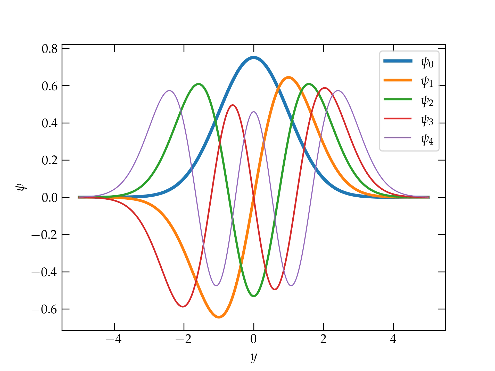
Figure 1 — The five lowest-energy normalized wave functions of a simple harmonic oscillator. Note that each successive wave function has one more node than the previous.
The next step is to investigate numerical approaches to solve the equation.