
A linear first-order differential equation has the form \begin{equation}\label{eq:DE1} \dv{y}{t} + p(t) y(t) = q(t) \end{equation} where \(t\) is the independent variable, \(y(t)\) is the dependent variable, and \(q(t)\) is a forcing function. If \(q(t) = 0\), the equation is homogeneous; if not, it is nonhomogeneous. For given functions \(p(t)\) and \(q(t)\), a solution requires the additional input of the value of \(y(t)\) at some chosen initial time (typically \(t = 0\)). Under general conditions we will outline below, the solution \(y(t)\) exists and is unique. In the following, I will typically use a prime to indicate differentiation with respect to the independent variable.
One strategy for finding \(y(t)\) is to seek to express the left-hand side of the equation as the total derivative of some function of \(t\).
We would like to know under what conditions a solution to the equation \(y' = f(t, y)\), with \(y(t_0) = y_0\) has a solution. The Existence and Uniqueness Theorem holds the following:
If \(f(t, y)\) and \(\pdv{f}{y}\) are continuous on a closed rectangle \(R\) on the \(ty\) plane and the point \((t_0, y_0)\) is inside \(R\), then a solution \(y(t)\) exists on some interval of \(t\) that contains \(t_0\) in its interior, and no more than one solution in \(R\) on any \(t\) interval that contains \(t_0\).
One way to visualize a first-order equation is to show the slope \(y' = f(t, y)\) as a function of \(t\) and \(y\) in a slope field. We start at a particular point on the \(ty\) plane and follow the local value of slope to determine how the value of \(y\) should change in the next small interval of time. This takes us to a new value of \(y\), from which we can determine a new value of slope and then a new value of \(y\), etc. The result is illustrated in in Figure 1.
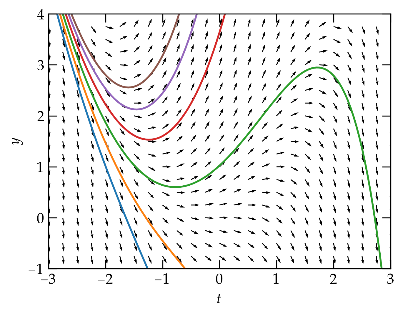
Figure 1 — The arrows show the derivative \(y'\); the smooth curves show example solutions to the first-order equation.
If the differential equation you seek to solve can be written in the form \begin{equation}\label{eq:separable} a(y) y’ + b(x) = 0 \end{equation} we can effectively separate the variables as follows. If \(A'(y) = a(y)\), then \begin{equation}\label{eq:dy} \dv{[A(y)]}{x} = \dv{A}{y} \dv{y}{x} = a(y) y’ \end{equation} by the chain rule. So, \begin{equation}\label{eq:sep} \dv{[A(y)]}{x} = - \dv{B}{x} = -b(x) \qquad\longrightarrow\qquad A(y) + B(x) = C \end{equation} for an integration constant \(C\). Note that this is the fussy mathematician’s way. Physicists are happy proceeding as follows: \begin{align} a(y) \dd{y} &= -b(x)\dd{x} \notag \\ \int a(y) \dd{y} &= \int -b(x)\dd{x} + C \end{align} Simple. The mathematicians have a point that you must be careful about “tearing apart a derivative” this way if you think it establishes a pattern that you can do the same thing with second-order derivatives, which you cannot!