
Consider the integral \[ I = \int_{-\infty}^{\infty} \frac{\sin^2 x}{x^2} \dd{x} \] whose integrand is shown in Fig.~1. Clearly, it is well-behaved at the origin, and finite, since it dies nicely for large \(|x|\). Can we use contour integration to evaluate it?
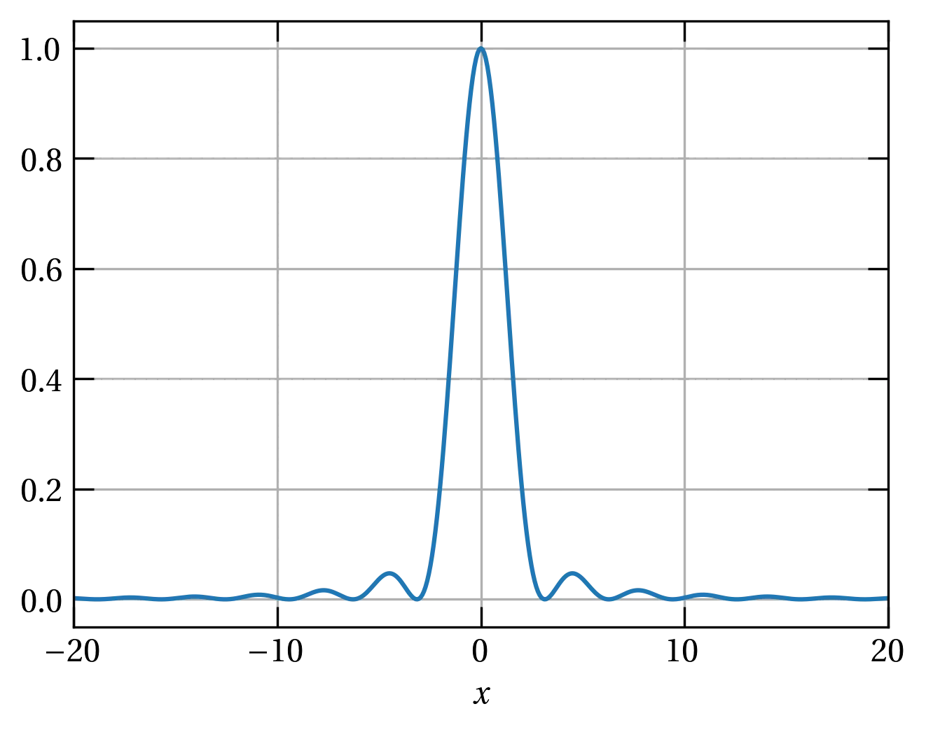
Figure 1 — A graph of \(\sin^2x / x^2\).
The first step is to express sine in terms of complex exponentials, \[ I = \int_{-\infty}^{\infty} \left(\frac{e^{iz} - e^{-iz}}{2iz} \right)^2 \dd{z} = \int_{-\infty}^{\infty} \frac{e^{2iz} - 2 + e^{-2iz}}{-4z^2}\dd{z} \] The first exponential will be well-behaved in the upper half-plane (UHP), whereas the second one will be well-behaved in the LHP. We’re going to have to break the integrand up to allow us to generate closed contours. So, we have \[ I = \int_{-\infty}^{\infty} \frac{1-e^{2iz}}{4z^2} \dd{z} + \int_{-\infty}^{\infty} \frac{1-e^{-2iz}}{4z^2} \dd{z} \] Both integrands have poles at \(z = 0\) which lie directly on the path of integration, so will only earn half the usual \(2\pi i a_{-1}\). However, each is a first-order pole, since the numerators are proportional to \(z\) for \(z \to 0\). Closing the contour for the first integral in a semicircle at \(R \to \infty\) in the UHP, it is straightforward to show that this addition adds nothing the integral, so its value will be \(\pi i a_{-1}\) as \(z \to 0\). The residue of the first integrand is \[ a_{-1}^+ = \lim_{z\to 0} z \frac{1 - (1 + 2iz + (2iz)^2/2! + \cdots)}{4z^2} = \lim_{z\to 0} - \frac{2iz^2}{4z^2} = \frac{1}{2i} \] and by similar argument, the residue of the second integrand is \(a_{-1}^- = -\frac{1}{2i}\). So, it might seem that they wipe each other out.
However, since we have to close the contour for the second integral in the LHP, we traverse the contour in the negative direction, so we get \(-\pi i\) times that residue, which means they reinforce each other. Hence, \[ I = \pi i \left(\frac{1}{2i} \right) - \pi \left(-\frac{1}{2i} \right) = \pi \]
The Riemann zeta function is \(\zeta(n) = \sum_{j=1}^\infty j^{-n}\). Can we evaluate the sum in closed form somehow using contour integration? This example exercises lots of the skills we’ve been working on in the course: series, series expansions, contour integration, and a third-order pole!
I’m going to focus at the moment on \(\zeta(2)\). If we could somehow arrange for a series of poles to lie on the positive real axis at the integers, with residues equal to \(1/n^2\), and then if we could find a suitable contour to evaluate the integral around, we might be able to sum the series.
My first idea was to try the integrand \[ \frac{1}{z^2 \sin \pi z} \] The denominator has a zero at each positive integer, producing a simple pole. Unfortunately, it has a problem of alternating signs. Consider the neighborhood of the pole at \(n\), where we might take \(z = n + \xi\): \[ \sin (\pi z) = \sin{(n+\xi)\pi} = \sin n\pi \cos\pi\xi + \cos n\pi \sin \pi\xi = (-1)^n \pi \xi \]
To get rid of the alternating signs, maybe we could use \[ \frac{\cos\pi z}{z^2 \sin \pi z} \] since the cosine in the numerator will also oscillate in sign, so it will remove the sign oscillation from the quotient. Of course, we’d have to calculate the residues to make sure we were properly accounting for factors of \(\pi\). But, assuming we sweat the details, it would appear that we might evaluate \(\zeta(2)\) by integrating around the contour shown in Fig. 2.
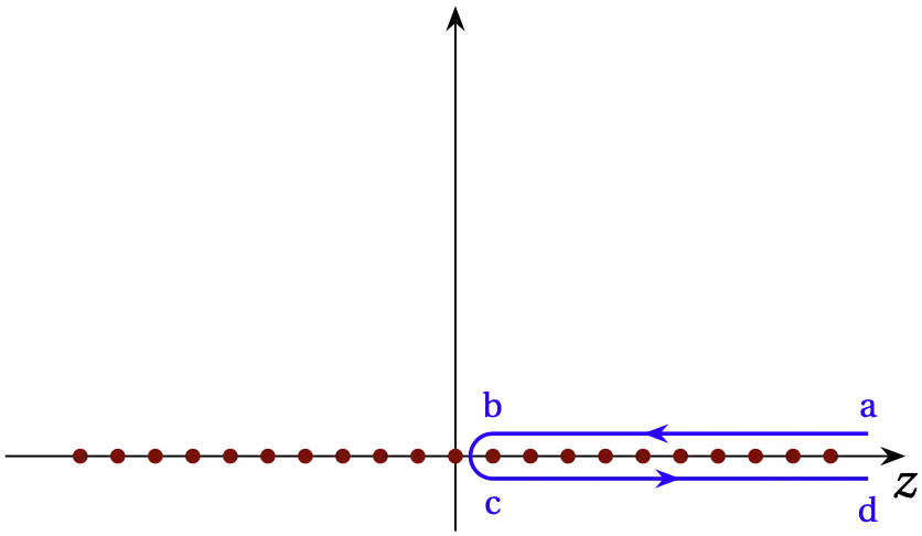
Figure 2 — Integrating around the illustrated contour in the positive sense would yield a value proportional to \(\zeta(2)\).
So, let’s now sweat the details by first calculating the residue of \(\cot\pi z/z^2\) at \(z = n\). The numerator goes to \(\cos \pi(n+\zeta) = \cos n\pi = (-1)^n\), and we already worked out that the denominator goes to \(n^2 \pi (-1)^n\). So, we need to multiply the integrand by \(\pi\) so that the residue is indeed the term we need to sum. That is \[ \zeta(2) = \frac{1}{2\pi i} \oint \pi\frac{\cot \pi z}{z^2} \dd{z} \] around the contour abcda.
By symmetry, all the poles on the negative real axis duplicate those enclosed in Fig. 2, so maybe we could consider the contour shown in Fig. 3.
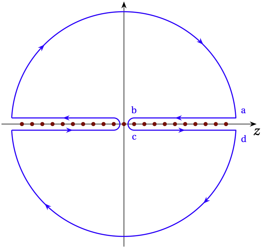
Figure 3 — A possible closed contour that might yield twice \(\zeta(2)\).
I know it looks crazy, but stay with me a moment. Let’s say for the sake of argument that the infinitesimal segment from d to a contributes nothing to the integral. If we could show that the contributions from the giant semicircles also vanish, then integrating around the contour in Fig. 3 should yield \(2 \zeta(2)\).
Along the semicircles, \(z = R e^{i\theta}\), so \(\dd{z} = i R e^{i\theta} \dd{\theta}\). Let’s think about the UHP first. That integral is \[ I_{\rm UHP} = \frac{1}{2\pi i}\int_{\pi}^0 \pi \frac{\cos \left[\pi R e^{i\theta}\right]}{R^2 e^{2i\theta} \sin\left[ \pi R e^{i\theta}\right]} i R e^{i\theta}\dd{\theta} = -\frac{1}{2 R} \int_0^\pi i \frac{e^{i\pi R (\cos\theta + i\sin\theta)} + e^{-i\pi R (\cos\theta + i\sin\theta)}}{e^{i\pi R (\cos\theta + i\sin\theta)} - e^{-i\pi R (\cos\theta + i\sin\theta)}} e^{-i\theta} \dd{\theta} \] In the upper half-plane, \(\sin\theta \ge 0\), so the second exponential in both numerator and denominator blow up in exactly the same way, while the first exponential goes strongly to zero. Multiplying numerator and denominator by \(e^{i\pi R(\cos\theta + i\sin\theta)}\) gives \begin{align} I_{\rm UHP} &= \frac{1}{2 i R} \int_0^\pi \frac{1 + e^{i 2\pi R(\cos\theta + i \sin\theta)}} {1 - e^{i 2\pi R(\cos\theta + i\sin\theta)}} e^{i\theta}\dd{\theta} \notag \\ &= \frac{1}{2 i R} \int_0^\pi \frac{1 + e^{-2\pi R \sin\theta} e^{i 2\pi R\cos\theta}} {1 - e^{-2\pi R \sin\theta} e^{i 2\pi R \cos\theta}} e^{i\theta}\dd{\theta} \notag \\ &= \frac{1}{2 i R} \int_0^\pi e^{i\theta}\dd{\theta} \notag \\ &= \frac{1}{2 i R} \frac{e^{i\pi} - e^0}{i} = \frac{1}{R} \end{align} Clearly, in the limit as \(R \to \infty\), \(I_{\rm UHP} \to 0\). The same argument applies to the semicircle in the lower half-plane. Therefore, the integral around the contour of Fig. 3 should yield \(2\zeta(2)\).
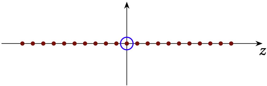
Figure 4 — Shrinking the contour from Figure 3 down to a tiny circle surrounding the pole at the origin.
We can now shrink the contour down to the tiny circle around the origin shown in Fig. 4, since the integrand is well-behaved throughout the region away from the real axis. Notice, however, that we are going around the pole at the origin in the negative direction, so \[ 2\zeta(2) = - 2\pi i a_{-1}(z = 0) \] All we have to do is evaluate the residue of \(\frac{1}{2\pi i} \pi\cot \pi z / z^2\) at \(z = 0\). We can do this using series expansions: \begin{align} \frac{1}{2\pi i} \pi \frac{\cot \pi z}{z^2} &= -\frac{i}{2z^2} \frac{1 - \pi^2 z^2 / 2! + \cdots} {\pi z - (\pi z)^3/3! + \cdots} \notag \\ &= - \frac{i}{2 \pi z^3} \frac{1 - \pi^2 z^2 / 2! + \cdots} {1 - (\pi z)^2/3! + \cdots} \notag \\ &= -\frac{i}{2\pi z^3} \left[1 - \frac{\pi^2 z^2}{2!} + \cdots \right] \left[1 + \frac{\pi^2 z^2}{3!} - \cdots \right] \notag \\ &= - \frac{i}{2\pi z^3} \left[ 1 - \frac{\pi^2 z^2}{3} + \cdots \right] \end{align} Hence, the residue is \(a_{-1} = i \pi / 6\) and \[ 2 \zeta(2) = - 2 \pi i \left(\frac{i \pi}{6} \right) \qquad\longrightarrow\qquad \boxed{ \zeta(2) = \frac{\pi^2}{6} } \] Kinda like magic!