
A Maclaurin series seeks to represent an arbitrary differentiable function, \(f(x)\), in a power series as \begin{equation} f(x) = f(0) + f’(0) x + \frac{f^{\prime\prime}(0)}{2!}x^2 + \cdots = \sum_{n=0}^\infty \frac{f^{(n)}(0)}{n!} x^n \end{equation} We showed that such series are unique, implying that the functions \(x^n\) are linearly independent basis vectors. What other functions might we use in a general series expansion? In particular, suppose that we are interested in representing periodic functions.
A periodic function with period \(T\) has the property that \[ f(t+T) = f(t) \] for all \(t\). You are already familiar with a large class of periodic functions, the trigonometric functions sine, cosine, and tangent, along with their reciprocals, but these just scratch the surface.
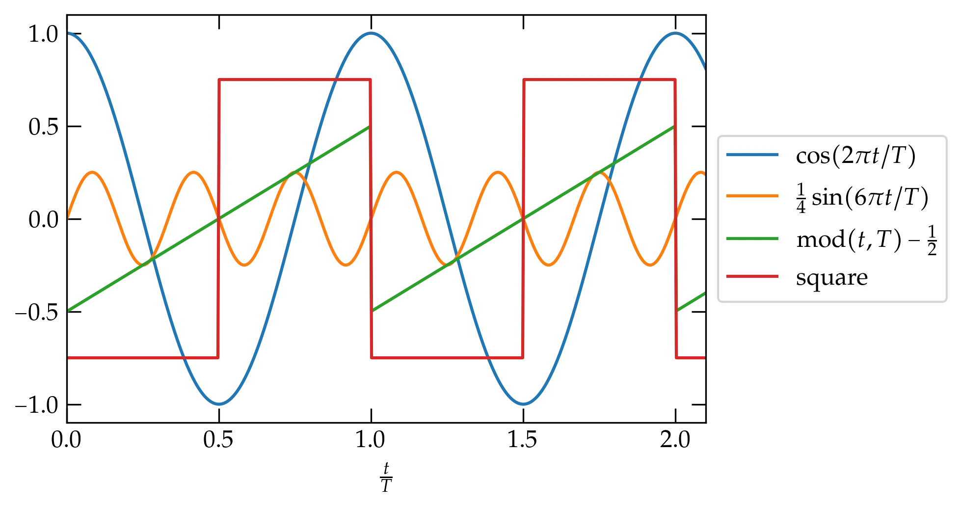
Figure 1 — A few functions with period \(T\).
Before we attack the general theory, I have to relate the most memorable “little trick” I learned in my first college math class, which is how to integrate \(\sin^2\theta\) and \(\cos^2\theta\) over convenient intervals. Of course, the general method that always works is to use the identities \[ \sin^2\theta = \frac{1 - \cos2\theta}{2} \qqtext{or} \cos^2\theta = \frac{1 + \cos 2\theta}{2} \] and actually perform the integration. However, as illustrated in Fig. 2, if the interval over which you integrate has symmetry such that \(\sin^2\theta\) and \(\cos^2\theta\) have the same area, then by the Pythagorean theorem, each must average to 1/2. Therefore, \begin{align} \int_0^T \sin^2 \left(\frac{2\pi t}{T}\right) \dd{t} &= \frac{T}{2} \notag \\ \int_0^T \cos^2 \left(\frac{2\pi t}{T}\right) \dd{t} &= \frac{T}{2} \notag \end{align}
Easy, peasy!!
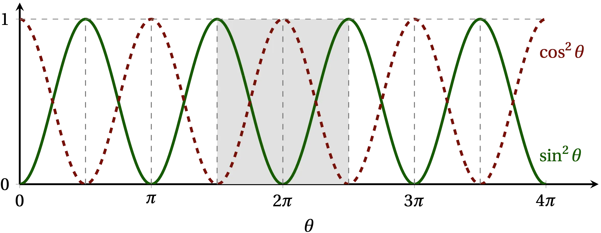
Figure 2 — Over the interval shaded in the figure, the area under the curves for \(\sin^2\theta\) and \(\cos^2\theta\) are the same, and since they sum to 1 by the Pythagorean theorem, \(\sin^2\theta + \cos^2\theta = 1\), each has the average value of 1/2.
Let \(f(t)\) be an arbitrary periodic function with period \(T\). Can we find a series representation of \(f(t)\) in terms of the very well-behaved trigonometric functions, sine and cosine? The most general combination of all sines and cosines with period \(T\) would have the form \begin{equation}\label{eq:fourierseries} f(t) = a_0 + \sum_{n=1}^\infty \qty[a_n \cos \qty(\frac{2 \pi n t}{T}) + b_n \sin \qty(\frac{2 \pi n t}{T})] \end{equation} where I have explicitly factored out the cosine term with \(n = 0\), and the coefficients \(a_n\) and \(b_n\) are as yet unknown. Apart from the leading constant, which represents the average value of the function, all terms in the series have frequencies that are integer multiples of the fundamental frequency, \(\nu = 1/T\). This form of series is called a Fourier series, and Fourier found a straightforward way to determine these unknown coefficients.
The method relies on a perhaps surprising but deep property of these trigonometric functions. Key points:
For these functions, we may define an inner product of the form \[ \ev{f,g} = \int_0^T f(t) g(t) \dd{t} \] and we may now show that the basis functions, \[ \sin\qty(\frac{2\pi n t}{T}) \qqtext{and} \cos\qty(\frac{2\pi n t}{T}) \] are orthogonal to one another with this definition of inner product. That is, \begin{align} \int_0^T \sin\qty(\frac{m 2\pi t}{T}) \sin\qty(\frac{n 2\pi t}{T}) \dd{t} &= \begin{cases} \frac{T}{2} & m = n \\ 0 & m \ne n \end{cases} \label{eq:sinsin} \\ \int_0^T \sin\qty(\frac{m 2\pi t}{T}) \cos\qty(\frac{n 2\pi t}{T}) \dd{t} &= 0 \\ \int_0^T \cos\qty(\frac{m 2\pi t}{T}) \cos\qty(\frac{n 2\pi t}{T}) \dd{t} &= \begin{cases} T & m = n = 0 \\ \frac{T}{2} & m = n > 0 \\ 0 & m \ne n \end{cases} \label{eq:thisone} \end{align} Can we prove these?
I will first prove Eq. \eqref{eq:sinsin} using “classic trig”. The proof relies on the trigonometric identity \begin{equation}\label{eq:cossum} \cos(\alpha \pm \beta) = \cos\alpha\cos\beta \mp \sin\alpha\sin\beta \end{equation} which is straightforward to prove using Euler’s identity, \[ e^{i \theta} = \cos\theta + i \sin\theta \] and letting \(\theta = \alpha \pm \beta\). Subtracting the sum formula from the difference gives \[ \cos(\alpha - \beta) - \cos(\alpha + \beta) = 2 \sin\alpha \sin\beta \] Therefore, \[ \int_0^T \sin\qty(\frac{m 2\pi t}{T}) \sin\qty(\frac{n 2\pi t}{T}) \dd{t} = \frac12 \int_0^T \qty[\cos\qty(\frac{(m-n)2\pi t}{T}) - \cos\qty(\frac{(m+n)2\pi t}{T}) ] \dd{t} \] The second term integrates to \[ -\frac12 \int_0^T \cos\qty(\frac{(m+n)2\pi t}{T}) \dd{t} = -\frac12 \qty[\frac{T}{(m+n)2\pi} \sin\qty(\frac{(m+n)2\pi t}{T})]_0^T = 0 \] since the integrated expression vanishes at both endpoints.
If \(m\ne n\) we get the same expression with \(m+n \to m-n\), which vanishes for the same reason. However, if \(m=n\), the first cosine term is just the constant 1, so it integrates to \(\frac{T}{2}\).
To illustrate an (allegedly) easier approach that uses complex exponentials, I will now attempt a proof of Eq. \eqref{eq:thisone}. To simplify the notation, I will use \(\omega = 2 \pi /T\). We will need to know how to evaluate the single (simple) integral for integral \(N\): \begin{equation}\label{eq:keyortho} I_N = \int_0^T e^{i N \omega t}\dd{t} = \begin{cases} t \bigg|_0^T = T & N = 0 \\ \displaystyle \frac{e^{iN\omega t}}{iN\omega} \bigg|_0^T = \frac{e^{i 2 \pi N} - 1}{i N \omega} = 0 & N \ne 0 \end{cases} \end{equation} That is, unless \(N = 0\), the integral vanishes, since we integrate over an integral number of complete periods, so the numerator is the same at the beginning and end of the integration. However, if \(N = 0\), the exponential is just 1, so we get an integral equal to the range of integration.
Then Eq. \eqref{eq:thisone} is \begin{align} \int_0^T \cos(m\omega t) \cos(n\omega t)\dd{t} &= \int_0^T \left(\frac{e^{im\omega t} + e^{-im\omega t}}{2} \right) \, \left( \frac{e^{in\omega t} + e^{-in\omega t}}{2}\right) \dd{t} \notag\\ &= \frac14 \int_0^T \bigg( e^{i(m+n)\omega t} + e^{i(m-n)\omega t} + e^{-i(m-n)\omega t} + e^{-i(m+n)\omega t} \bigg) \dd{t} \end{align} By Eq. \eqref{eq:keyortho}, the only integrals that are nonzero have \(m\pm n = 0\). There are three cases. If \(m = n = 0\), then all four terms yield \(T/4\) and the integral evaluates to \(T\). If, however, \(m = n \ne 0\), then only two terms yield \(T/4\), so the integral evaluates to \(T/2\). Finally, if \(m \ne n\), then all the terms vanish and the integral evaluates to 0.
The strategy for determining the coefficients \(a_n\) and \(b_n\) in Eq. \eqref{eq:fourierseries} is now clear. To deduce \(b_m\), multiply Eq. \eqref{eq:fourierseries} by \(\sin(m 2 \pi t/T)\) and integrate over a full period. The only term that survives on the right-hand side has coefficient \(b_m\). Therefore, \begin{equation}\label{eq:bn} b_m = \frac{2}{T} \int_0^T \sin\qty(\frac{m 2 \pi t}{T}) f(t) \; dt \end{equation}
By similar reasoning, we get that \begin{align} a_0 &= \frac{1}{T} \int_0^T f(t) \; dt \label{eq:a0} \\ a_m &= \frac{2}{T} \int_0^T \cos \qty(\frac{m 2 \pi t}{T}) f(t) \; dt \qquad m > 0 \label{eq:an} \end{align}
Let’s see if we can determine the Fourier series for the square wave defined on the interval \(-\frac{T}{2} \le t < \frac{T}{2}\) by \begin{equation}\label{eq:square} f(t) = \begin{cases} -1 & -\frac{T}{2} \le t < 0 \\ +1 & 0 < t < \frac{T}{2} \end{cases} \end{equation} and periodic with period \(T\).
Consider first the cosine terms given by Eqs. \eqref{eq:a0} and \eqref{eq:an}. All of them are even functions on this interval, \(f(-t) = f(t)\), whereas \(f(t)\) is odd, \(f(-t) = -f(t)\). Their product, therefore, is odd and integrates to zero. Hence, \(a_n = 0\) by symmetry for all \(n\).
What about for the sine terms? All of them are odd, so we can’t use the same symmetry argument to get rid of them. However, the product of two odd functions is an even function, and so it will suffice to double the value of the integral of Eq. \eqref{eq:bn} over the range \(0 \le t \le T/2\) to solve for \(b_n\): \begin{align} b_n &= 2 \times \frac{2}{T} \int_0^{T/2} \sin\qty(\frac{2\pi n t}{T})\;dt \notag \\ &= \frac{4}{T} \; \left. -\frac{T}{2\pi n} \cos\qty(\frac{2\pi n t}{T})\;dt \right|_0^{T/2} \notag \\ &= \frac{2}{n\pi} \qty[1 - \cos(n\pi)] \notag \end{align} When \(n\) is even, this expression vanishes; when \(n\) is odd, it equals 2. So, we have determined that \[ \boxed{ f(t) = \frac{4}{\pi} \sum_{n = 1}^\infty \frac1n \sin\qty(\frac{ 2\pi n t}{T}) \qquad (n\text{ odd}) } \]
What does this look like? To get some idea, we can truncate the infinite sum at a finite number of terms and get a sense for how it is converging. We can use the following bit of Python code to create a plot:
t = np.linspace(-0.5,0.5,341)
fig, ax = plt.subplots()
ω = 2*np.pi
curves = (3, 11, 31, 101)
y = np.zeros(len(t))
for n in range(1, 102, 2):
    y += 4/(n*np.pi) * np.sin(ω*n*t)
    if n in curves:
        ax.plot(t, y, label=r"$n = %d$" % n)
ax.set_xlabel("$t / T$")
ax.legend();
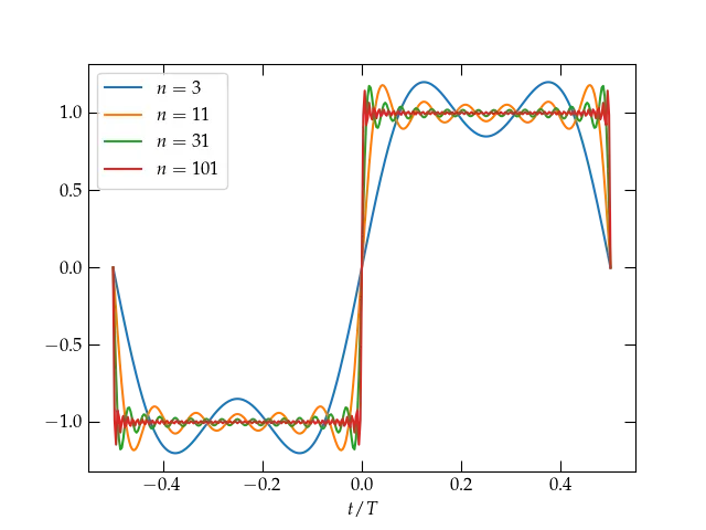
Figure 3 — The Fourier series representation of the square wave defined in Eq. \eqref{eq:square} for terms through the given order \(n\). Increasing numbers of terms allow the series to approach ever more closely the constant value 1 for \(0 < t < \frac{T}{2}\), but there appears to be a persistent overshoot at the discontinuities, which is called the Gibbs phenomenon.
Stopping after just two terms (\(n=3\)) does not make a very convincing representation of the square wave, but as we add more and more terms, it does indeed appear that the Fourier series is at least trying to converge to \(f(t)\), at least away from its points of discontinuity. Let’s home in on the region around \(t = 0\).
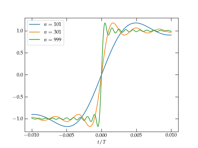
Figure 4 — At the point of discontinuity at \(t = 0\), the series is clearly converging to the midpoint between the limit values on either side. As the number of terms increases, the transition from \(-1\) to \(1\) grows narrower, but the Gibbs overshoot phenomenon persists. See this page for more on the Gibbs phenomon.
The rate of convergence of this series is quite slow (the coefficients are proportional to \(1/n\)) because of the discontinuity at \(t = 0\) and the endpoints. We can explore the rate of convergence by investigating a continuous function that lacks a continuous first derivative, such as a triangular wave given by \[ g(t) = \frac12 - \frac{2|t|}{T} \qquad -\frac{T}{2} \le t \le \frac{T}{2} \] for which the Fourier series is \[ g(t) = \frac{8}{\pi^2} \sum_{n\text{ odd}} \frac{\cos (n \omega t)}{n^2} \] Now the coefficients fall off like \(1/n^2\), much faster than for the square wave.
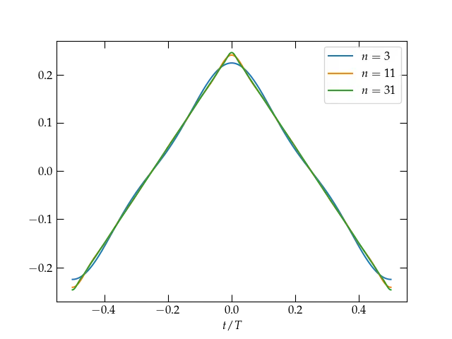
Figure 5 — Truncated Fourier series approximation to a sawtooth wave. Comparing the rate of convergence to the discontinuous square wave, it clearly takes many fewer terms for the Fourier series to converge to this continuous function that lacks a continuous first derivative. The coefficients
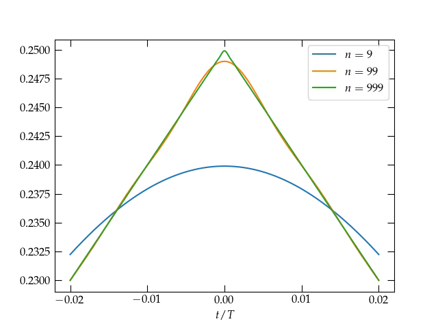
Figure 6 — Near a point of discontinuity in the first derivative, the rate of convergence is slower, although still significantly faster than in the first example.
To demonstrate that the sines and cosines are orthogonal over a period, we took advantage of trigonometric identities. We now seek to develop an approach that relies only on the governing differential equation and doesn’t need such specialized knowledge as trig identities.
The trigonometric functions satisfy the differential equation \begin{equation}\label{eq:DE} u^{\prime\prime}(x) = \lambda u(x) \end{equation} for a (negative) constant \(\lambda\). Consider two such solutions, \(u_1^{\prime\prime} = \lambda_1 u_1\) and \(u_2^{\prime\prime} = \lambda_2 u_2\). Now form the quantity \begin{equation} \label{eq:towardBC} (u_1^{\prime\prime})^* u_2 - (u_1)^* u_2^{\prime\prime} = \lambda_1^* u_1^* u_2 - u_1^* \lambda_2 u_2 = (\lambda_1^* - \lambda_2) u_1^* u_2 \end{equation} and integrate from \(a\) to \(b\): \begin{align} \int_a^b [(u_1^{\prime\prime})^* u_2 - (u_1)^* u_2^{\prime\prime} ] dx &= (\lambda_1^* - \lambda_2) \int_a^b u_1^* u_2 \dd{x} \notag \\ \left[ (u_1^{\prime})^{*} u_2 - u_1^* u_2^\prime \right]_a^b - \int_a^b \left[ (u_1^{\prime})^{*} u_2^{\prime} - (u_1^{\prime})^{*} u_2^{\prime}\right] \dd{x} &= (\lambda_1^* - \lambda_2) \int_a^b u_1^* u_2 \dd{x} \notag \\ \left[ u_1^{\prime*} u_2 - u_1^* u_2^\prime \right]_a^b &= (\lambda_1^* - \lambda_2) \int_a^b u_1^* u_2 \dd{x} \end{align}
The term on the left is called the bilinear concomitant. If we use the boundary condition \(u(a) = 0\) or \(u'(a) = 0\), and similarly at \(x = b\), then the bilinear concomitant vanishes. Another way to make it vanish is with periodic boundary conditions, in which \(u(a) = u(b)\) and \(u'(a) = u'(b)\).
Let us suppose that we do indeed impose such boundary conditions that make the bilinear concomitant vanish. If \(u_2(x) = u_1(x)\), then we get \begin{equation}\label{eq:BC0} 0 = (\lambda_1^* - \lambda_1) \int_a^b |u_1(x)|^2 \, dx \end{equation} Unless \(u_1(x) = 0\), the integral is positive definite, which implies that \(\lambda_1\) must be real.
Now let \(\lambda_1\) differ from \(\lambda_2\). Then \begin{equation}\label{eq:orthogonal} 0 = (\lambda_1^* - \lambda_2) \int_a^b u_1^* u_2 \, dx = (\lambda_1^* - \lambda_2) \langle u_1, u_2 \rangle \end{equation} Since, by assumption, the eigenvalues differ, the integral (inner product) must vanish. That is, the eigenfunctions corresponding to different eigenvalues are orthogonal, in the sense defined by Eq. \eqref{eq:orthogonal}.
What functions satisfy the differential equation Eq. \eqref{eq:DE} and the boundary conditions \(u(0) = 0\) and \(u'(L) = 0\)? Cosine functions are nonzero at the origin, so the boundary condition there rules them out. We must have \begin{equation}\label{eq:exa} u_n(x) = \sin \left[ \left(n+\frac12 \right)\frac{\pi x}{L} \right] \qquad\text{for } n \in \mathbb{Z} \end{equation} These functions are orthogonal on the interval \([0,L]\) and can be used to represent an arbitrary function on that interval.
As an example, suppose we use a parabolic arc that vanishes at the origin and has zero slope at \(L\): \begin{equation}\label{eq:fx} f(x) = 1 - \left(\frac{L-x}{L}\right)^2 = \frac{2x}{L} - \frac{x^2}{L^2} \end{equation}
Using the orthogonality of the functions defined in Eq. \eqref{eq:exa}, you can show that \begin{equation}\label{eq:result} f(x) = \sum_{n = 0}^\infty \frac{32}{\pi^3 (1+2n)^3} \sin\left[\left(n+\frac12\right)\frac{\pi x}{L}\right] \end{equation}
As is apparent in Figure 7, the series converges extremely rapidly, since the basis function with \(n = 0\) is a pretty close approximation to the parabola.
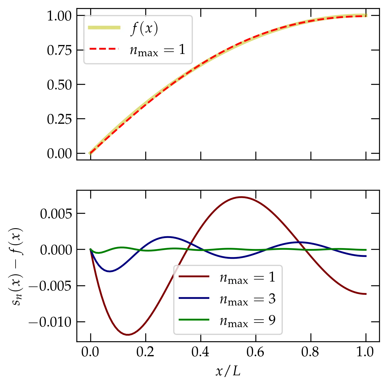
Figure 7 — Convergence of the Fourier series representation of the parabolic function defined in Eq. \eqref{eq:fx}. The top panel shows the true function and the Fourier approximation that uses only the terms with \(n=0\) and \(n=1.\) The bottom panel shows the difference between the truncated series and the true function for different points of truncation.
The convergence of the previous example seems a bit too good. What happens if we ask the Fourier series to converge to a function that is inconsistent with the boundary conditions we have imposed? Suppose, for instance, that we use the same basis functions of Eq. \eqref{eq:exa} to represent a parabola that peaks not at \(x = L\) but in the middle of the range? The result is \begin{equation}\label{eq:awk} g(x) = \frac{4}{L^2} x (L-x) = \sum_{n=0}^\infty \frac{16 - 8 \pi (n+\frac12) (-1)^n}{[\pi(n+\frac12)]^3} \sin\left[\pi \left(n+\frac12 \right)\frac{x}{L}\right] \end{equation} which is illustrated in Figure 8.
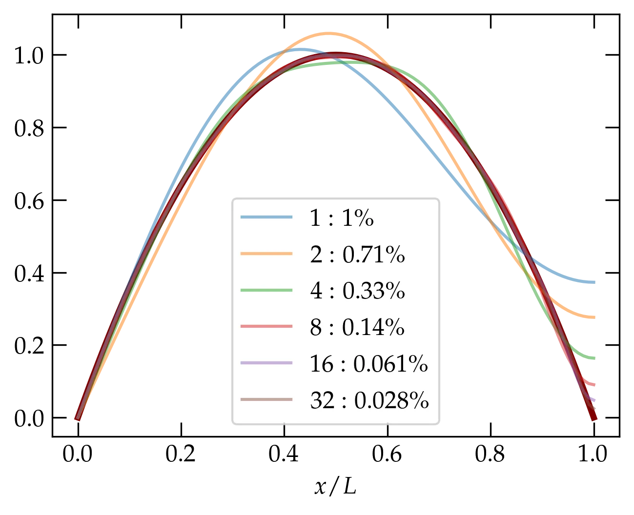
Figure 8 — Convergence of the Fourier series using basis functions to represent a parabola that is symmetric in the interval \([0, L]\). The percentage shown in the legend is the value of \(\sqrt{ \langle f-s_n, f-s_n\rangle }\).
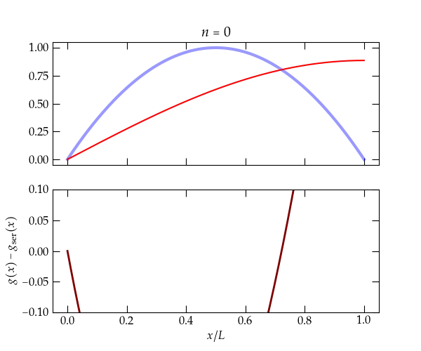
Figure 9 — Same as above, but showing versions of the series through increasing number of terms. The series converges more slowly than the parabola that agrees with the boundary conditions. Note the additional power of \(n\) in the numerator.
When the bilinear concomitant vanishes, we are guaranteed that basis eigenfunctions \(u_n(x)\) corresponding to different eigenvalues \(\lambda_n\) are orthogonal: \(\ev{u_m, u_n} = 0\) when \(m \ne n\). Let us also assume that we have normalized the basis functions so that \begin{equation}\label{eq:normalization} \ev{u_m, u_n} = \delta_{mn} \end{equation} (Remember that our inner product is defined as \(\ev{u_m, u_n} = \int_a^b u_m^*(x) u_n(x) \dd{x}\).) That is, the functions \(u_n\) form an orthonormal basis for functions on the interval \(a \le x \le b\), which means that we can represent an arbitrary function \(f(x)\) as \begin{equation}\label{eq:arbf} f(x) = \sum_{n} a_n u_n(x) \end{equation} and we can evaluate the coefficients \(a_n\) via \(a_n = \ev{u_n, f}\). Put another way, \begin{equation}\label{eq:compact} f(x) = \sum_n \ev{u_n, f} u_n(x) \end{equation} which is precisely parallel to using an orthonormal basis of \(\mathbb{R}^n\) via \begin{equation}\label{eq:vector} \va{r} = \sum_n \ev{\vu{e}_n, \va{r}} \vu{e}_n \end{equation}
Compute \begin{align} \int_a^b |f(x)|^2 \dd{x} &= \int_a^b \dd{x} \left[ \sum_m a_m u_m(x) \right]^* \left[ \sum_n a_n u_n(x) \right] \notag \\ \ev{f,f} &= \sum_{m,n} a_m^* a_n \ev{u_m, u_n} = \sum_n |a_n|^2 \ev{u_n, u_n} \notag \\ \ev{f,f} &= \sum_n |a_n|^2 \label{eq:Prseval} \end{align} The last line, \eqref{eq:Prseval}, is Parseval’s identity. As a mathematical result, it is akin to the Pythagorean theorem; we add up the squares of the components of a vector and we get its magnitude squared. But, it also has an important physical interpretation. The energy in an oscillatory function (a wave) is proportional to its amplitude squared. The coefficients \(|a_n|^2\) represent the energy in each basis function.