
The imaginary unit was conjured to be able to solve \(z^2 = x\) for all \(x \in \mathbb{R}\). The cheapest extension to the real numbers is to define \(i = \sqrt{-1}\) and to represent an arbitrary complex number as \[ z = x + iy\qquad x,y \in \mathbb{R} \] Here \(x\) represents the real part of \(z\) and \(y\) the imaginary part of \(z\). The algebra of the two parts is just the algebra of the real numbers, so addition is commutative. As for multiplication of two complex numbers, we have \begin{align} (x_1 + i y_1)\times (x_2 + i y_2) &= x_1 x_2 + x_1 i y_2 + i y_1 x_2 + i^2 y_1 y_2 \notag\\ &= (x_1 x_2 - y_1 y_2) + i(x_1 y_2 + y_1 x_2) \notag \end{align} Both the real and imaginary parts of the product are unchanged on exchanging 1 and 2; multiplication of complex numbers is also commutative.
There are more involved ways to solve \(z^2 = x\) that preserve the commutative property of addition but not for multiplication. In particular, the quaternions are defined by \begin{align} -1 &= i^2 = j^2 = k^2 \notag \\ i j &= k = - j i \qqtext{and cyclic permutations}\notag \end{align} The quaternions have three distinct square roots of \(-1\), and the products of these roots are antisymmetric; the multiplication of quaternions does not commute. Although Gauss invented them (for himself), William Rowan Hamilton (after whom the hamiltonian is named) independently developed them and spent much of his career developing their properties. Quaternions were all the rage when James Clerk Maxwell was working out electromagnetic theory and figure prominently in his treatise. Before long, Josiah Willard Gibbs and Oliver Heaviside developed vector notation and the quaternions were shelved, by and large, although they can be very convenient for representing rotations in three-dimensional space. Out of fondness for quaternions, mathematicians persist in using \(\vb{i}\), \(\vb{j}\), and \(\vb{k}\) for unit vectors in the \(x\), \(y\), and \(z\) directions, respectively, but that’s just silly and certainly does not generalize to the curvilinear coordinate systems that play such an important role in physics.
A common way to visualize complex numbers is on the Argand plane, in which the real part of the number is plotted on the \(x\) axis and the imaginary part along the \(y\) axis.
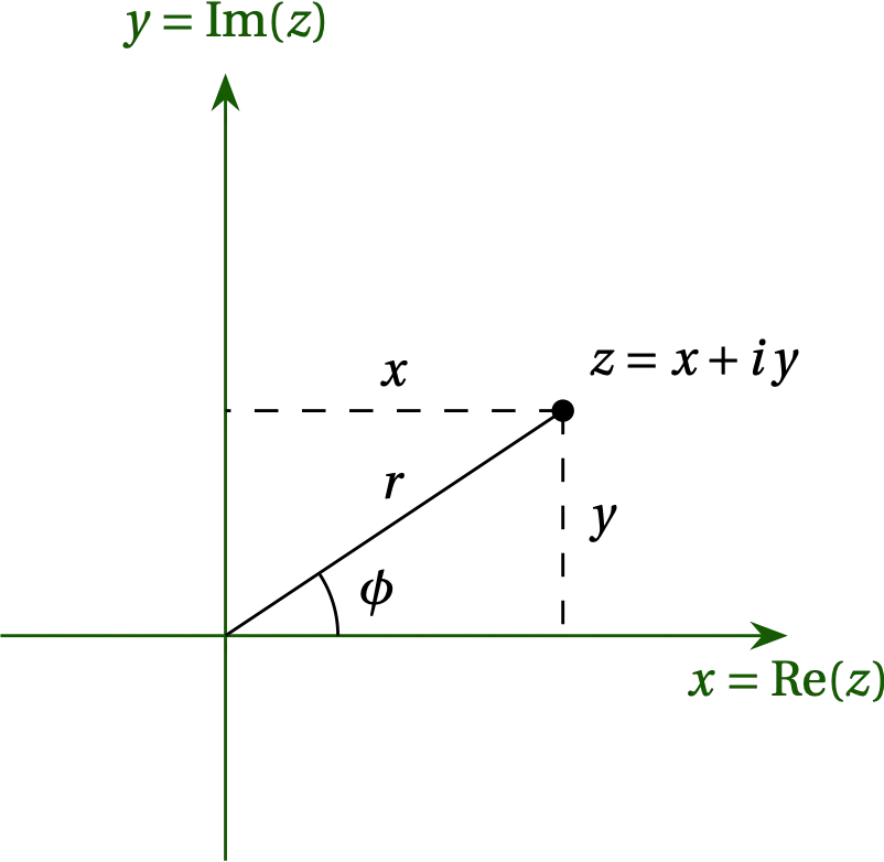
Figure 1 — The complex number \(z = x + i y\) (for real \(x\) and \(y\)) is plotted on the \(xy\) plane at point \((x,y)\).
Of course, we could also use a polar coordinate system in which \begin{align} r &= \sqrt{x^2 + y^2} = |z| & \qquad x &= r \cos\phi = \Re(z) \notag \\ \phi &= \arctan(y/x) &\qquad y &= r \sin\phi = \Im(z) \notag \end{align} Using Euler’s identity, \begin{equation}\label{eq:Euler} e^{i \phi} = \cos\phi + i \sin\phi \end{equation} we have \[ z = r e^{i\phi} \] for the polar representation of the complex number \(z\).
Addition is straightforward when complex numbers use the rectangular (Cartesian) representation, but the expression for the product of complex numbers is more involved. On the other hand, products and quotients of complex numbers are simple in polar form, but addition and subtraction are more involved.
Euler’s identity allows us to represent sines and cosines in terms of complex exponentials: \begin{align} \cos\phi &= \frac{e^{i\phi} + e^{-i\phi}}{2} = \Re(e^{i\phi}) \notag \\ \sin\phi &= \frac{e^{i\phi} - e^{-i\phi}}{2i} = \Im(e^{i\phi}) \notag \end{align} The complex representation makes it easy to work out trigonometric identities. For example, \begin{align} e^{i\theta} e^{i\phi} = e^{i(\theta+\phi)} &= \cos(\theta+\phi) + i \sin(\theta+\phi) \notag \\ (\cos\theta + i \sin\theta)(\cos\phi+i\sin\phi) &= \cos(\theta+\phi) + i \sin(\theta+\phi) \notag \\ (\cos\theta\cos\phi - \sin\theta\sin\phi) + i(\sin\theta\cos\phi + \cos\theta\sin\phi) &= \cos(\theta+\phi) + i \sin(\theta+\phi) \notag \end{align} therefore by comparing real and imaginary parts on both sides, we have \begin{align} \cos(\theta+\phi) &= \cos\theta\cos\phi - \sin\theta\sin\phi \notag \\ \sin(\theta+\phi) &= \sin\theta\cos\phi + \cos\theta\sin\phi \end{align}
Or another: \begin{align} \cos^4\theta &= \frac{(e^{i\theta} + e^{-i\theta})^4}{2^4} = \frac{e^{4i\theta} + 4 e^{2i\theta} + 6 + 4e^{-2i\theta}+e^{4i\theta}}{16}\notag \\ &= \frac18 \cos 4\theta + \frac12 \cos 2\theta + \frac38 \end{align} You can confirm the plausibility of this last identity by checking out \(\theta \in \{0, \frac\pi2, \pi\}\).
Next: Fourier Series