
We saw on the previous page that the Fourier series for a square wave overshot the mark at the point of discontinuity at \(t = 0\) where the square wave jumps from \(-1\) to \(1\), as illustrated in Fig. 1.
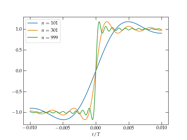
Figure 1 — At the point of discontinuity at \(t = 0\), the series is clearly converging to the midpoint between the limit values on either side. As the number of terms increases, the transition from \(-1\) to \(1\) grows narrower, but the Gibbs overshoot phenomenon persists.
Is there a way to quantify this overshoot?
Recall that we found that the series representing the square wave is \begin{equation}\label{eq:squarewave} f(t) = \frac{4}{\pi} \sum_{n\text{ odd}}^\infty \frac1n \sin\qty(\frac{ 2\pi n t}{T}) \end{equation}
It would be nice if we could convert this trigonometric series to a geometric series, which would make it easier for us to manipulate. Can we do that?
From Euler’s formula, \(e^{i \phi} = \cos\phi + i \sin\phi\), we could rewrite this series as \begin{equation}\label{eq:sw2} f(t) = \frac{4}{\pi} \Im \sum_{n\text{ odd}} \frac{1}{n} e^{i n \omega t} \end{equation} where I have let \(\omega = 2 \pi / T\) for notational convenience.
If we could get rid of the \(1/n\) term inside the sum, we would have a geometric series. Suppose we take a time derivative of \(f(t)\). Just to be sure we don’t run into any issues as the upper limit of the sum tends to infinity, let us use an explicit upper limit. That is, let \begin{equation}\label{eq:g} g_N(t) = \frac{4}{\pi} \Im \sum_{m = 0}^N \frac{1}{1 + 2m} e^{i(1+2m)\omega t} \end{equation} so that \(f(t) = \lim_{N \to \infty} g_N(t)\). There is no problem differentiating the finite series \(g_N(t)\): \begin{equation}\label{eq:gprime} g’_N(t) = \frac{4}{\pi} \Im \sum_{m = 0}^N i \omega e^{i(1+2m)\omega t} = \frac{4\omega}{\pi} \Im \left( ie^{i\omega t} \sum_{m=0}^N e^{i 2 m \omega t} \right) \end{equation} The series is geometric, with ratio \(r = e^{2i\omega t}\); we know how to sum such series! \begin{equation}\label{eq:gprimesum} g’_N(t) = \frac{4 \omega}{\pi} \Im \left( ie^{i\omega t} \frac{1 - e^{i 2(N+1) \omega t}}{1 - e^{2i\omega t}} \right) \end{equation} It is often handy to symmetrize the numerator and denominator, which we could do by factoring out \(e^{i(N+1)\omega t}\) from the numerator and \(e^{i\omega t}\) from the denominator: \[ g’_N(t) = \frac{4\omega}{\pi} \Im \left( i e^{i\omega t} \frac{e^{i(N+1)\omega t}}{e^{i\omega t}} \frac{e^{-i(N+1)\omega t} - e^{i(N+1)\omega t}}{e^{-i\omega t} - e^{i\omega t}} \right) = \frac{4\omega}{\pi} \Im \left( i e^{i(N+1)\omega t} \frac{\sin(N+1)\omega t}{\sin \omega t} \right) \] The sine terms are clearly real, so the imaginary part of the term in large parentheses is \[ g’_N(t) = \frac{4\omega}{\pi} \cos(N+1)\omega t \frac{\sin(N+1)\omega t}{\sin\omega t} = \frac{2\omega}{\pi} \frac{\sin2(N+1)\omega t}{\sin\omega t} \]
The first peak for \(t > 0\) will be when \(\sin 2(N+1)\omega t = 0\) or \(2(N+1)\omega t = \pi\), so \[ t_\text{peak} = \frac{\pi}{2(N+1)\omega} = \frac{T}{4(N+1)} \]
We now can integrate \(g'_N(t)\) from zero to \(t_\text{peak}\) to see how large the overshoot goes. \[ g_N(t_\text{peak}) = \int_0^{t_\text{peak}} \frac{4}{T} \frac{\sin 2(N+1)\omega t}{\sin\omega t}\dd{t} = \frac{4}{T} \int_0^{x_\text{peak}} \frac{\sin 2(N+1)x}{\sin x} \frac{\dd{x}}{\omega} \] where \(x_\text{peak} = \omega t_\text{peak} = \frac{2\pi}{T} \frac{T}{4(N+1)} = \frac{\pi}{2(N+1)}\). For \(N \gg 1\), \(x_\text{peak} \ll \pi\). Throughout the range of integration, \(\sin x \approx x\). So, \[ g_N(t_\text{peak}) \approx \frac{2}{\pi} \int_0^{\frac{\pi}{2(N+1)}} \frac{\sin2(N+1)x}{x} \dd{x} \] We can rewrite this a bit by letting \(y = 2(N+1)x\), so that \begin{equation}\label{eq:gNt} g_N(t_\text{peak}) \approx \frac{2}{\pi} \int_0^{\pi} \frac{\sin y}{y}\dd{y} \end{equation} Note that all dependence on \(N\) has dropped out, provided that \(N\) is large enough to allow the denominator to be approximated as \(x\).
I can’t do this integral analytically, although the sine integral is defined by \[ \mathrm{Si}(x) \equiv \int_0^x \frac{\sin t}{t}\dd{t} \] in terms of which, \[ g_\text{peak} \approx \frac{2}{\pi} \mathrm{Si}(\pi) \]
We can also use scipy to do the integral numerically:
from scipy.integrate import quad
(val, err) = quad(lambda x : 1 if x == 0 else np.sin(x) / x, 0, np.pi)
2 * val / np.pi
1.1789797
So, the height of the peak should be 1.179, which does indeed seem to be consistent with Fig. 2.
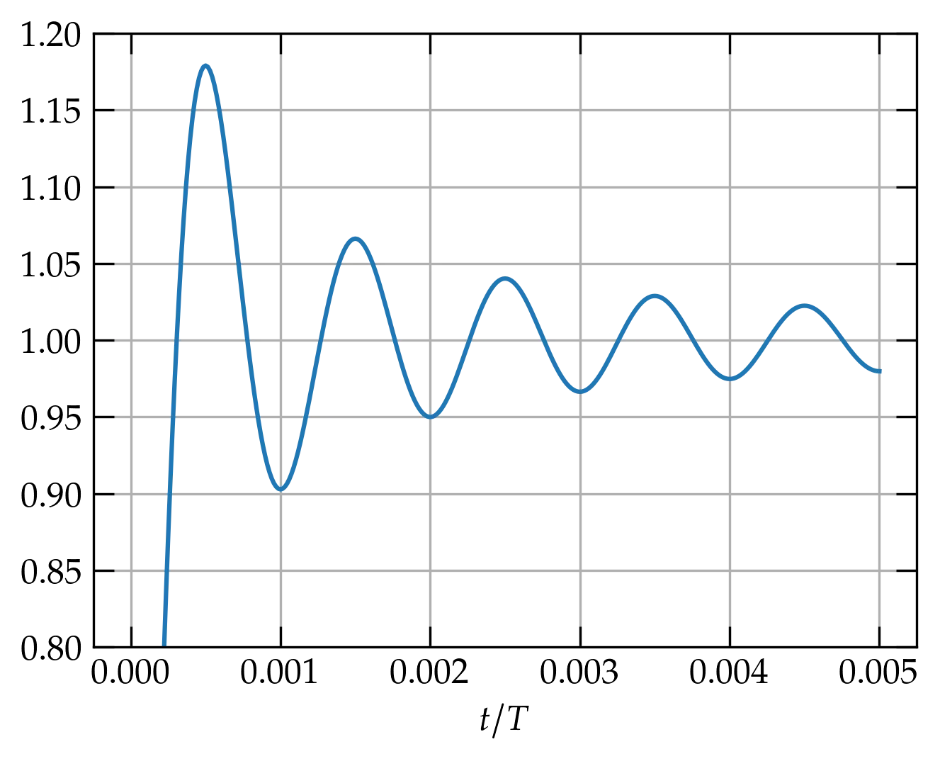
Figure 2 — Zooming in on the Gibbs peak near \(t = 0\), using a sum through \(N=999\). The peak does indeed seem consistent with \(\frac{2}{\pi} \text{Si}(\pi) \approx 1.179\).