
An infinite series is an infinite sum, \begin{equation}\label{eq:infseries} s = \sum_{n=1}^{\infty} a_n = \lim_{N\to\infty} \sum_{n=1}^N a_n \end{equation} that is the limit of partial sums having a finite number of terms. For the limit to exist, the magnitude of the terms \(a_n\) must go to zero as \(n\to\infty\). However, while this is a necessary condition it is not sufficient. The harmonic series, \[ H = \sum_{n=1}^{\infty} \frac1n = 1 + \frac12 + \frac13 + \cdots \] does not converge, even though its terms tend to zero as \(n \to \infty\). Its divergence is logarithmic (i.e., weak), as illustrated in the following figure
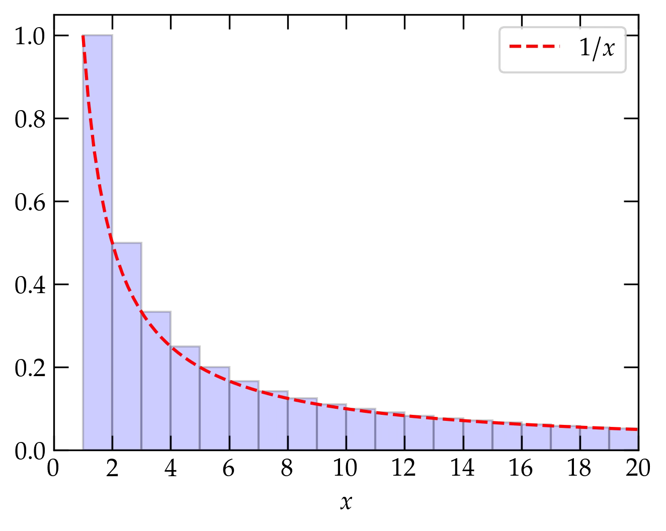
Figure 1 — The harmonic series is represented by the area shaded blue of the bars of height \(1\), \(\frac12\), \(\frac13\), etc. The area of the bars is greater than the area under the curve \(1/x\) (shown in red), since the curve is everywhere contained within a bar. Since \(\int_1^x \frac1{x'}\dd{x'} = \ln x\), which slowly diverges as \(x\to\infty\), the harmonic series diverges even though its individual terms tend to zero.
Successive terms of a geometric series form a fixed ratio \(r\): \[ S_N = a_0(1 + r + r^2 + \cdots r^N) = \sum_{n=0}^N a_0 r^n \] There is a nifty trick for summing a (finite) geometric series. Consider \(r S_N\): \begin{align} S_N &= a_0 (1 + r + r^2 + \cdots + r^N) \\ r S_N &= a_0(\hphantom{1 + } \;\, r + r^2 + \cdots + r^N + r^{N+1}) \end{align} If we now subtract the second line from the first, we get \begin{equation} \label{eq:geo} S_N (1-r) = a_0 (1 - r^{N+1}) \qquad\text{so}\qquad \boxed{ S_N = a_0 \left( \frac{1 - r^{N+1}}{1 - r} \right) } \end{equation}
The series converges to \(S_{\infty} = \frac{a_0}{1-r}\) as \(N\to\infty\), provided that \(|r| < 1\) (so that the numerator of the fraction goes to 1). Sometimes it is convenient to symmetrize this expression by factoring out \(r^{N/2}\), which allows you to express the fraction in terms of the ratio between hyperbolic sine functions.
It is often necessary to know whether an infinite series converges to a finite value. Some of the useful tests to answer this question are:
Use numpy to confirm Eq. (\ref{eq:geo}) for \(r = 0.99\) and \(N=100\).
Does the series \(\displaystyle \sum_{n=2}^{\infty} \frac{1}{n \ln n}\) converge?
(a) Show that the series \(\displaystyle \sum_{n=2}^\infty \frac{1}{n(\ln n)^2}\) converges. (b) Use numpy to sum the terms through \(n = 100,000\). You should get 2.022 883 9. (c) Use an integral to obtain the sum of the infinite series to six significant figures.
Does the series \(\displaystyle \sum_{n=1}^{\infty} \frac{1}{n(n+1)}\) converge? If it does, can you sum it?
The Riemann zeta function is defined by \begin{equation}\label{eq:zeta} \zeta(\nu) = \sum_{n=1}^\infty \frac1{n^{\nu}} \end{equation} If \(\nu=1\), this series becomes the harmonic series, which we know to be divergent. For \(\nu < 1\) it diverges more rapidly, but for \(\nu > 1\) we can use an integral test to check convergence: \[ \zeta(\nu) = \sum_{n=1}^\infty \frac1{n^{\nu}} < 1 + \int_2^{\infty} (x-1)^{-\nu} \dd{x} = 1 + \left.\frac{(x-1)^{1-\nu}}{1-\nu}\right|_{x=2}^{\infty} = 1 + \frac{1}{\nu-1} = \frac{\nu}{\nu-1} < \infty \qquad\text{when } \nu > 1 \]
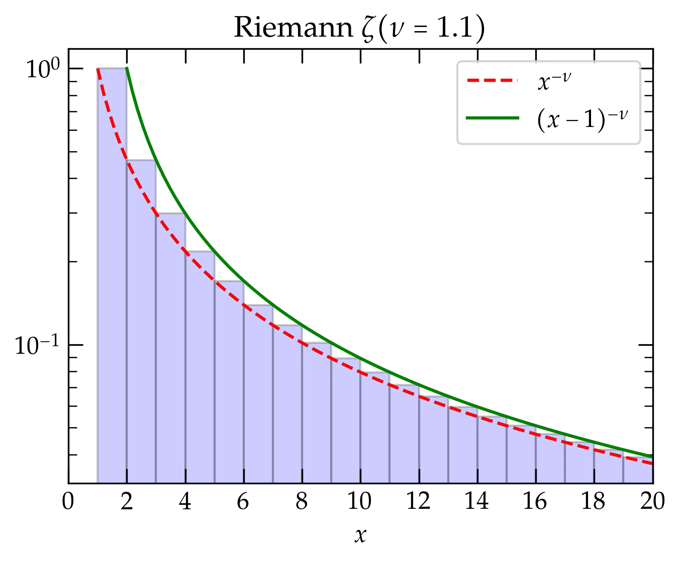
Figure 2 — The Riemann zeta function for \(\nu = 1.1\). The red and green curves clearly bound the area of the blue bars, which represents the Riemann \(\zeta\) for \(\nu = 1.1\) (note the logarithmic vertical scale).
The Riemann zeta function pops up occasionally in physics, including the theory of blackbody radiation and the determination of the Stefan-Boltzmann constant, \(\sigma\), which relates the power per unit area radiated by an ideal blackbody at temperature \(T\): \begin{equation}\label{eq:Stefan-Boltzmann} p = \sigma T^4 \qquad\text{where}\qquad \sigma = \frac{6 \zeta(4) k_{\mathrm{B}}^4}{\pi^2 c^2 \hbar^3} = \frac{2 \pi^5 k_{\mathrm{B}}^4}{15 c^2 h^3} \approx 5.67 \times 10^{-8}\,\mathrm{W \cdot m^{-2} \cdot K^{-4}} \end{equation}
If successive terms in a series alternate sign, and if the magnitude of the terms goes to zero as \(n\to\infty\), then the series converges. An infinite series is absolutely convergent if the sum of the absolute value of its terms converges. If the series converges, but it is not absolutely convergent, it is called conditionally convergent.
Properties of absolutely convergent series:
Note that none of these claims can be made for conditionally convergent series.
Taylor’s expansion is a way of approximating a function \(f(x)\) in the neighborhood of a point \(x=a\) with a polynomial in powers of \((x-a)\) such that the first \(n\) derivatives of the polynomial match the first \(n\) derivatives of \(f(x)\) at \(a\), \begin{equation} \label{eq:Taylor} f(x) \approx f(a) + (x-a) f’(a) + \frac{(x-a)^2}{2!} f^{\prime\prime}(a) + \cdots + \frac{(x-a)^n}{n!} f^{(n)}(a) \end{equation} where the inequality comes from ignoring higher-order terms.
A useful way to bound the error associated with ignoring those terms is to integrate the \(n\)th derivative from \(a\) to \(x\) \(n\) times: \begin{align} \int_a^{x_{n-1}} f^{(n)} \dd{x_n} &= f^{(n-1)}(x_{n-1}) - f^{(n-1)}(a) \notag \\ \int_a^{x_{n-2}} \dd{x_{n-1}} \int_a^{x_{n-1}} \dd{x_{n}} f^{(n)}(x_n) &= f^{(n-2)}(x_{n-2}) - f^{(n-2)}(a) -(x_{n-2} - a) f^{(n-1)}(a) \notag \\ \vdots \qquad & \qquad \vdots \notag \\ &= f(x) - f(a) -(x-a) f’(a) - \frac{(x-a)^2}{2!} f^{\prime\prime}(a) - \cdots - \frac{(x-a)^{n-1}}{(n-1)!} f^{(n-1)}(a) \end{align} Rearranging slightly gives \begin{equation}\label{eq:Taylor2} f(x) = \sum_{i=0}^{n-1} \frac{(x-a)^i}{i!} f^{(i)}(a) + R_n \end{equation} where the remainder is the \(n\)-dimensional integral, \[ R_n = \int_a^x \dd{x_1} \cdots \int_a^{x_{n}} \dd{x_n} \; f^{(n)}(x_n) = \frac{(x-a)^n}{n!} f^{(n)}(\xi) \] for some value \(a \le \xi \le x\) by the mean value theorem. Equation (\ref{eq:Taylor2}), with the explicit form of the residual \(R_n\) is a particularly powerful way of not only estimating functions but also the magnitude of the error associated with a finite series.
Physicists should know the following series cold; they arise very frequently in physics and it is worth your time to learn so well that you don’t need to think about them. (Actually, each of these is a Maclaurin series, which is a form of Taylor series in which the derivatives are evaluated at \(a = 0\)):
\begin{align} e^x &= 1 + x + \frac{x^2}{2!} + \frac{x^3}{3!} + \frac{x^4}{4!} + \cdots & &-\infty < x <\infty \notag \\ \sin x &= x - \frac{x^3}{3!} + \frac{x^5}{5!} - \frac{x^7}{7!} + \cdots & &-\infty < x <\infty \notag \\ \cos x &= 1 - \frac{x^2}{2!} + \frac{x^4}{4!} - \frac{x^6}{6!} + \cdots & &-\infty < x <\infty\notag \\ \sinh x &= x + \frac{x^3}{3!} + \frac{x^5}{5!} + \frac{x^7}{7!} + \cdots & &-\infty < x <\infty \notag \\ \cosh x &= 1 + \frac{x^2}{2!} + \frac{x^4}{4!} + \frac{x^6}{6!} + \cdots & &-\infty < x <\infty\notag \\ \frac{1}{1-x} &= 1 + x + x^2 + x^3 + x^4 + \cdots & & -1 < x < 1 \notag \\ \ln(1+x) &= x - \frac{x^2}{2} + \frac{x^3}{3} - \frac{x^4}{4} + \cdots & &-1 < x \le 1 \notag \\ (1+x)^n &= 1 + n x + \frac{n(n-1)}{2!} x^2 + \frac{n(n-1)(n-2)}{3!} x^3 + \cdots & & -1 < x < 1 \tag{binomial} \end{align} Clearly, the radius of convergence of the logarithmic series does not include \(x = -1\), which generates a divergent harmonic series. For the binomial series, the series terminates when \(n\) is a positive integer and so converges for all \(x\). When \(n\) is not a positive integer, the series does not terminate and may not converge.
Taylor series offer a useful alternative to l’Hôpital’s rule for evaluating the limit of the ratio of two functions, \(f(x)\) and \(g(x)\), both of which tend to zero as \(x \to x_0\). As an example, consider \[ L = \lim_{x\to0} \frac{1 - \cos x}{x^2} \] where \(f(x) = 1 - \cos x\) and \(g(x) = x^2\), both of which go to zero as \(x \to 0\). To evaluate using l’Hôpital’s rule, form \(f'(x)/g'(x)\): \[ L = \lim_{x\to0} \frac{f’(x)}{g’(x)} = \lim_{x\to0} \frac{\sin x}{2x} \] That’s still indeterminate, in the form \(0/0\), so we can apply l’Hôpital’s rule once again to get \[ L = \lim_{x\to0}\frac{f^{\prime\prime}(x)}{g^{\prime\prime}(x)} = \lim_{x\to0}\frac{\cos x}{2} = \frac12 \]
Alternatively, we can use the Taylor series for \(\cos x\): \[ L = \lim_{x\to0} \frac{1 - (1 - x^2/2! + x^4/4! - \cdots)}{x^2} = \lim_{x\to0} \frac{1}{2!} - \frac{x^2}{4!} + \cdots = \frac12 \] No need to compute derivatives (if you already know the Taylor series)! Oftentimes, this approach is much simplier than (successive) “trips to the hospital.”
Suppose that you knew a Maclaurin series for a function \(f(x)\) but you need the series for \(1/f(x)\), valid for small values of \(x\). For example, we know the series for \(\cosh x\) from the above list (or we could derive it ourselves). The hyperbolic secant function, \(\sech x = 1 / \cosh x\). How could we compute the series for \(\sech x\), valid for small \(x\) through terms of order \(x^6\)?
The “easy” way is to go back to the definition in Eq. (\ref{eq:Taylor}) and work out all the derivatives of \(\sech(x)\). While this is straightforward, in principle, the expressions for the derivatives get more and more complicated as we proceed. [If you don’t believe me, try it!]
Here’s another option. For small \(x\), \begin{equation} \cosh x = 1 + \underbrace{\frac{x^2}{2!} + \frac{x^4}{4!} + \frac{x^6}{6!} + \cdots}_{q} \end{equation} where \(q\) is a “small quantity” as long as \(x\) isn’t too large. So, \begin{equation}\label{eq:sech1} \sech x = \frac{1}{\cosh x} = \frac{1}{1 + q} = (1 + q)^{-1} \end{equation} But, the binomial series for \(n = -1\) is just \[ \frac{1}{1 + q} = 1 - q + q^2 - q^3 + \cdots \] To produce the series for \(\sech x\) valid for terms through \(x^6\) just requires us to keep all the terms in \(-q + q^2 - q^3\) through \(x^6\). We’ll work term by term: \begin{align} -q &= -\frac{x^2}{2!} - \frac{x^4}{4!} - \frac{x^6}{6!} - \frac{x^8}{8!} + \O{x^{10}} \notag \\ q^2 &= \frac{x^4}{(2!)^2} + 2 \frac{x^2 \; x^4}{2! \; 4!} + 2 \frac{x^2}{2!} \frac{x^6}{6!} + \left( \frac{x^4}{4!} \right)^2 + \O{x^{10}} \notag \\ &= \frac{x^4}{4} + \frac{x^6}{4!} + x^8 \left( \frac{1}{6!} + \frac{1}{(4!)^2} \right) + \O{x^{10}} \notag \\ -q^3 &= -\left(\frac{x^2}{2!} \right)^3 - 3 \left(\frac{x^2}{2!}\right)^2 \frac{x^4}{4!} + \O{x^{10}} \notag \\ q^4 &= \frac{x^8}{16} + \O{x^{10}} \notag \end{align}
Now, we just need to combine all these terms: \begin{align} \sech x &= 1 - \frac{x^2}{2} + x^4 \left( -\frac{1}{4!} + \frac{1}{4} \right) + x^6 \left( -\frac{1}{6!} + \frac{1}{4!} - \frac{1}{8} \right) \notag \\ &\qquad + x^8 \left( -\frac{1}{8!} + \frac{1}{6!} + \frac{1}{(4!)^2} - \frac{1}{32} + \frac{1}{16} \right) + \O{x^{10}} \notag \\ &= 1 - \frac{x^2}{2} + \frac{5 x^4}{24} - \frac{61 x^6}{720} + \frac{277 x^8}{8064} + \O{x^{10}} \end{align}
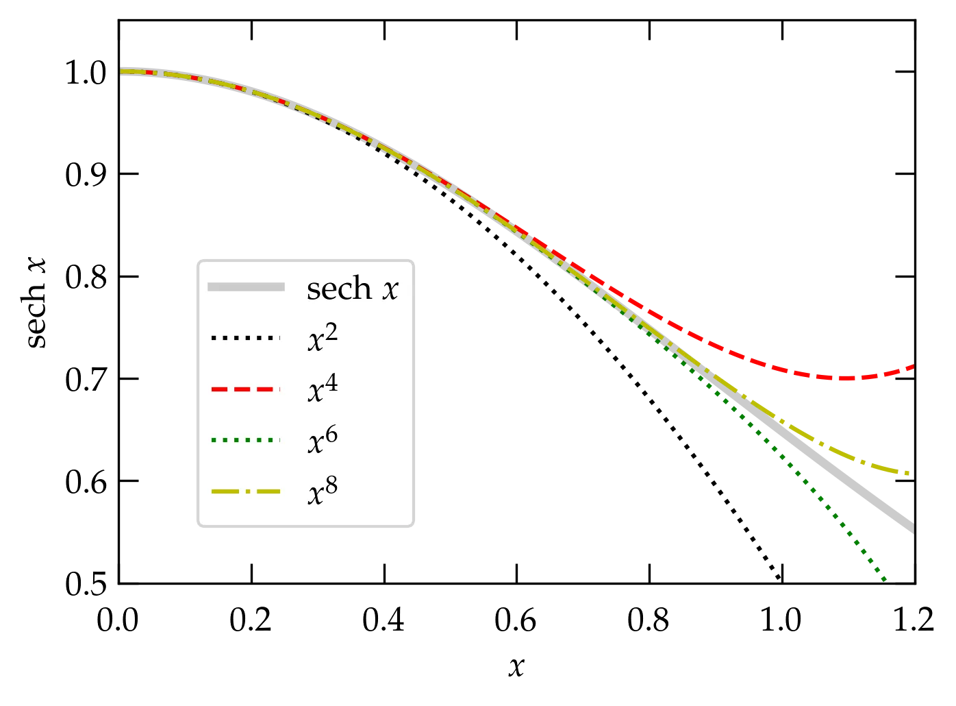
Figure 3 — Maclaurin series for the hyperbolic cosine obtained by inverting the series for \(\cosh x\). Each successive curve includes the terms through the order listed in the legend.
See the page on Euler’s \(\Gamma\) function for an illustration of the power of series expansion as a means of obtaining an analytic expression for the factorial function.
Derive a power series expansion through \(x^5\) for \(\cot x\) by dividing the series for \(\cos x\) by the series for \(\sin x\). Ans: \[ \cot x = \frac1x - \frac{x}{3} - \frac{x^3}{45} - \frac{2 x^5}{945} + \cdots \] Note that this series includes a negative power of \(x\), which means it is not a Taylor series. Series that include negative powers are called Laurent series and are very common in the theory of functions of a complex variable.
The derivative of \(\tan^{-1}x\) is \((1+x^2)^{-1}\). By integrating, find a series expansion for \(\tan^{-1} x\).
One way to compute a series for \(\sin^{-1} x\) is to start with \(x = \sin y\). Then $$dx/dy =
Unless Vatche provides a reasonable justification, I suspect I’ll omit this section!
The Bernoulli numbers \(B_n\) arise in many computational physics problems; they may be defined by \[ \frac{t}{e^t-1} = \sum_{n=0}^\infty \frac{B_n t^n}{n!} \] One way to work out the first few Bernoulli numbers is to multiply both sides by \((e^t-1)/t\) to get \begin{align} 1 &= t^{-1} \qty(e^t - 1) \qty(B_0 + B_1 t + \frac{B_2 t^2}{2!} + \cdots) \notag \\ 1 &= \qty(1 + \frac{t}{2!} + \frac{t^2}{3!} + \cdots)\qty(B_0 + B_1 t + \frac{B_2 t^2}{2!} + \cdots) \notag \end{align} The only term on the right that has \(t^0\) in it is \(B_0\), so we deduce that \(B_0 = 1\). There are two terms that involve \(t^1\), which gives \[ 0 = B_0 \frac{t}{2} + B_1 t = \qty(\frac{B_0}{2} + B_1)t \longrightarrow B_1 = -\frac12 \] Gathering terms proportional to \(t^2\) yields \[ 0 = \qty(\frac{B_0 }{3!} + \frac{B_1}{2!} + \frac{B_2}{2!} )t^2 = \qty( \frac16 - \frac14 + \frac{B_2}{2})t^2 \longrightarrow B_2 = \frac16 \]
A routine to compute the first \(n\) Bernoulli numbers is available in scipy.special.bernoulli:
from scipy.special import bernoulli

bernoulli(6)
array([ 1.        , -0.5       ,  0.16666667,  0.        , -0.03333333,
        0.        ,  0.02380952])
As you can probably guess from this output, the Bernoulli numbers for odd \(n \ge 3\) all vanish.

Figure 4 — Geometry of Fresnel diffraction, where \(|x| \ll s_0\) and the cosine of the angle between \(s_0\) and \(x\) is \(x_s / s_0\).
Compute \(s - s_{0}\) to second order in \(x\), where the law of cosines gives \begin{equation} s^{2} = s_{0}^{2} + x^{2} - 2 x x_{s} \end{equation} and \(x_{s}\) is a constant. That is, you may ignore terms proportional to \(x^{3}\) or any higher power of \(x\).