
NumPy uses the @ operator to perform matrix multiplication. Given that
\[
\mat{m} = \begin{pmatrix} 1 & 2 \\ 3 & 4 \end{pmatrix}
\qquad\text{and}\qquad
\vb{v} = \begin{pmatrix} -2 \\ 1 \end{pmatrix}
\]
Then we would expect
\[
\mat{m}\vdot\mat{m} = \begin{pmatrix} 1 & 2 \\ 3 & 4 \end{pmatrix} \vdot \begin{pmatrix} 1 & 2 \\ 3 & 4 \end{pmatrix} = \begin{pmatrix} 7 & 10 \\ 15 & 22\end{pmatrix}
\]
\[
\mat{m}\vdot\vb{v} = \begin{pmatrix} 1 & 2 \\ 3 & 4 \end{pmatrix} \vdot \begin{pmatrix} -2 \\ 1 \end{pmatrix}
= \begin{pmatrix} 0 \\ -2 \end{pmatrix}
\]
\[
\vb{v} \vdot \mat{m} = \begin{pmatrix}-2 & 1\end{pmatrix}\vdot\begin{pmatrix} 1 & 2 \\ 3 & 4 \end{pmatrix} = \begin{pmatrix} 1 & 0 \end{pmatrix}
\]
\[
\vb{v} \vdot \vb{v} = 5
\]
m = np.array([[1, 2], [3, 4]])
array([[1, 2],
       [3, 4]])

m @ m
array([[ 7, 10],
       [15, 22]])

v = np.array([-2, 1])
array([ -2, 1])

m @ v
array([ 0, -2])

v @ m
array([1, 0])

v @ v
5
The generic matrix inversion routine in NumPy is numpy.linalg.inv:
np.linalg.inv(m)
array([[-2. ,  1. ],
       [ 1.5, -0.5]])
You can check that the inverse has been computed correctly (up to numerical rounding error):
m @ np.linalg.inv(m)
array([[1.00000000e+00, 0.00000000e+00],
       [1.11022302e-16, 1.00000000e+00]])
You can get both the eigenvalues and the corresponding normalized eigenvectors by calling np.linalg.eig(m).
evals, evecs = np.linalg.eig(m)
(evals, evecs)
(array([-0.37228132,  5.37228132]),
array([[-0.82456484, -0.41597356],
       [ 0.56576746, -0.90937671]]))
We can confirm that the eigenvectors are normalized and that they are indeed eigenvectors
np.linalg.norm(evecs, axis=0)
array([1., 1.])

evals[0] * evecs[:,0], m @ evecs[:,0]
(array([ 0.30697009, -0.21062466]), array([ 0.30697009, -0.21062466]))
The Cholesky decomposition of a positive-definite symmetric (Hermitian) square matrix factors the matrix into a lower-triangular matrix \(\mat{L}\) such that the matrix product \(\mat{L} \vdot \mat{L}^{\rm H}\) gives the original matrix, and where \(^{\rm H}\) denotes the Hermitian conjugate (the conjugate transpose). For a real matrix, it is just the transpose.
The matrix \[ \mat{n} = \begin{pmatrix} 2 & -1 & 0 \\ -1 & 2 & -1 \\ 0 & -1 & 2 \end{pmatrix} \] may be Cholesky decomposed to give \[ \mat{L} = \begin{pmatrix} \sqrt{2} & 0 & 0 \\ -\frac{1}{\sqrt{2}} & \sqrt{\frac32} & 0 \\ 0 & -\sqrt{\frac23} & \frac{2}{\sqrt{3}} \end{pmatrix} \]
n = np.array([[2, -1, 0], [-1, 2, -1], [0, -1, 2]])
ch = np.linalg.cholesky(n)
ch
array([[ 1.41421356,  0.        ,  0.        ],
       [-0.70710678,  1.22474487,  0.        ],
       [ 0.        , -0.81649658,  1.15470054]])

ch @ ch.T
array([[ 2., -1.,  0.],
       [-1.,  2., -1.],
       [ 0., -1.,  2.]])
According to Numerical Recipes, for matrices admitting a Cholesky decomposition, this method of solving \(\mat{A}\vdot\vb{x} = \vb{b}\) is more numerically stable and about a factor of 2 faster than standard LDU decomposition.
The singular value decomposition of a rectangular matrix \(\mat{M}\) takes the form \begin{equation} \mbox{\Large \(\underbrace{\mat{M}}_{m\times n} = \underbrace{\mat{u}}_{m\times m} \vdot \underbrace{\mat{S}}_{m\times n} \vdot \underbrace{\mat{v}^{\rm H}}_{n\times n}\) } \end{equation} where \(\mat{u}\) is unitary, \(\mat{S}\) is diagonal with the singular values in descending order along the main diagonal (and zeros elsewhere), and \(\mat{v}^{\rm H}\) is also unitary.
sm = np.array([[1, 2, 3, 4],
              [-4, 2, 7, 8]])
u, s, vh = np.linalg.svd(sm, full_matrices=False)

u
array([[-0.38930378, -0.92110942],
       [-0.92110942,  0.38930378]])

s
array([12.46596449,  2.75676067])

vh
array([[ 0.26433044, -0.21023856, -0.61091761, -0.71603689],
       [-0.8989988 , -0.38581923, -0.0138575 , -0.20676711]])

u @ np.diag(s) @ vh
array([[ 1.,  2.,  3.,  4.],
       [-4.,  2.,  7.,  8.]])
What is this good for? I’ll offer an example from image processing inspired by this page.
As the matrix to analyze via singular value decomposition, we will use the grayscale values of this \(522 \times 400\) pixel image of Harvey Seeley Mudd shown in Figure 1.
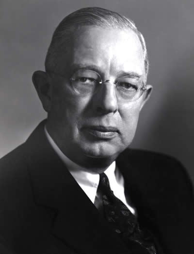
Figure 1 — Mining engineer and philanthropist Harvey Seeley Mudd.
The following Python script loads the image, converts it to grayscale, and then performs a singular value decomposition. To generate a compressed rendering using the \(k\) largest singular values, we use first \(k\) columns of \(\\\mat{U}\), the top-left \(k\) rows and columns of \(\mat{S}\), and the first \(k\) rows of \(\mat{V}^{\mathrm{T}}\).
harvey = plt.imread('Harvey-Mudd.jpg') # this is an RGB image
harvey = harvey[:,:,0] # convert to grayscale

from scipy.linalg import svd
U, S, V_T = svd(harvey, full_matrices=False)
S = np.diag(S)

fig, ax = plt.subplots()
k = 5
harvey_approx = U[:, :k] @ S[:k, :k] @ V_T[:k, :]
ax.imshow(harvey_approx, cmap='gray')
ax.set_title(r"$k = %d$" % k)
ax.axis('off')
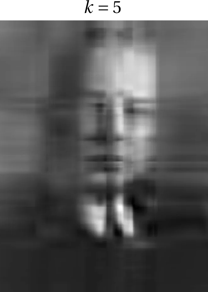

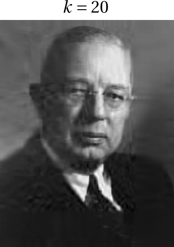


Figure 2 — approximations to the original “matrix” keeping only the \(k\) strongest singular values. The final image is the original.