
Stochastic processes have an essential component of randomness (the word stochastic comes from the Greek for “aim at, guess”).
Suppose that a walker of indeterminate gender begins at the origin and at each time step flips a coin; if it is heads, they take one step to the right; if it is tails, they take one step to the left. If we treat each coin flip as a random event (as opposed to a determinstic exercise in rotational and translational dynamics), then the “progress” that our walker makes away from the origin is a matter of probabilities. How far from the origin is the walker after \(N\) flips?
Such a random walk is described by the binomial distribution, for which the mean number of steps to the right is \(\ev{n} = N p\), where \(p\) is the probability of a step to the right (i.e., of the coin showing heads) and the standard deviation of the distance from the origin is \(\sigma = \sqrt{N p q}\), where \(q = 1 - p\). If the coin is fair, \(p = q = 1/2\) and the average position of the walker is the always at the origin, while the typical distance from the origin is \(\sigma = \frac12 \sqrt{N}\). That is, the typical net distance the random walker covers grows with the square root of the number of steps.
Use the rng.choice((-1,1), size=<n>) function call, along with np.cumsum to plot the displacement of a random walker taking steps of size 1 with equal probability in the positive and negative directions in a one-dimensional random walk and compare with binomial probability expectations.
Suppose that we now grant our inebriated random walker the flexibility of taking a random step of length 1 in any direction in the \(xy\) plane. How far do we expect them to get from the origin after \(N\) steps?
If each direction is equally likely, then the average value of \(\delta x\) for one step is \[ \ev{\delta x} = \frac{1}{2\pi} \int_0^{2\pi} \cos \theta \dd{\theta} = 0 \] and \[ \ev{(\delta x)^2} = \frac{1}{2\pi} \int_0^{2\pi} \cos^2 \theta\dd{\theta} = \frac12 \] The averages for \(\delta y\) are the same. So, after \(N\) steps, we expect \[ \ev{r^2} = N\ev{(\delta x)^2} + N\ev{(\delta y)^2} = \frac{N}{2} + \frac{N}{2} = N \] In other words, we expect the walker to be about at radius \(r = \sqrt{N}\) after \(N\) steps.
Simulate a random walk in which the walker takes random steps of length 1 in an arbitrary direction in the \(xy\) plane and see if you can corroborate the expectation that the walker is about \(\sqrt{N}\) steps from the origin after taking \(N\) steps. I say about, because our method evaluates the mean square distance, \(\ev{r^2}\). The average of \(r^2\) is greater than the square of the average of \(r\).
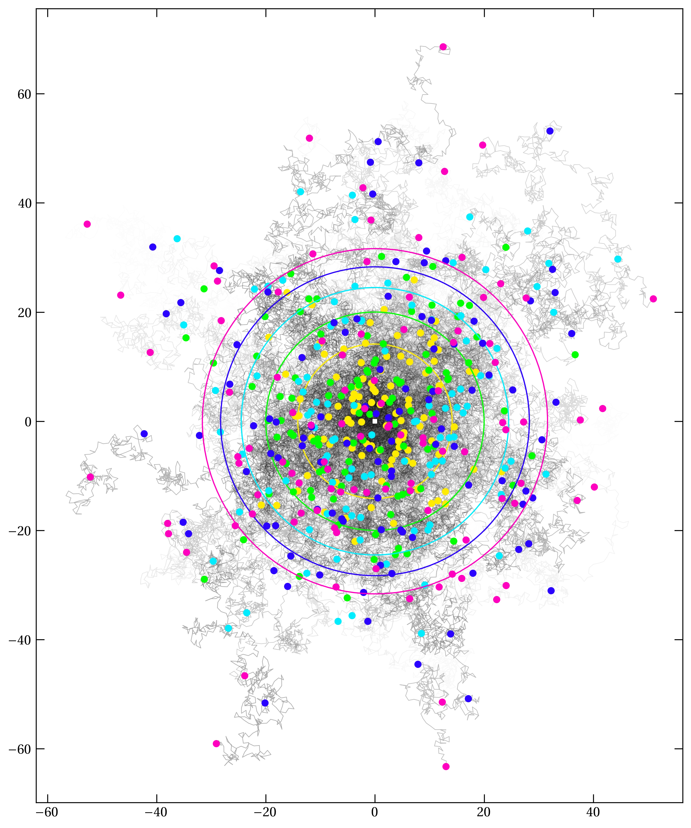
Figure 1 — A collection of two-dimensional random walks, starting from the origin (shown with a white square), each taking \(N=1000\) steps of unit length. The colored circles mark the expected value of \(\sqrt{\ev{r^2}} = \sqrt{n}\) after 200, 400, 600, 800, and 1000 steps. The colored dots make the corresponding position on each walk.
In mechanics we often simplify systems by ignoring their surroundings: for example, we ignore air resistance, friction at the pivot of a pendulum, and various other physical effects that we hope are small and don’t alter the system “too much.” If the system of interest can exchange energy with its surroundings, and the surroundings have temperature \(T\), then the probability of finding the system in a particular configuration (called a microstate) is proportional to the Boltzmann factor, \(e^{-E/k_{\rm B}T}\), where \(E\) is the system’s energy in the microstate, \(T\) is the absolute temperature (kelvins), and \(k_{\rm B}\) is the Boltzmann constant. As we have seen in my molecular dynamics simulation, even without an external thermal bath at temperature \(T\), when particles can exchange energy with one another and you have more than a few, the same dependence of microstate probability on the Boltzmann factor may be observed.
A general feature of systems of many particles (or degrees of freedom, meaning dynamical variables or coordinates) is that the number of microstates is an extremely rapidly increasing function of energy. As time evolves, the system moves from state to state, exploring a large number of accessible microstates. However, the number of microstates it can explore in a reasonable time is an infinitesimal fraction of all accessible microstates. When we measure some property of the system over an interval of time, we record a time-average. The ergodic hypothesis holds that the time average should give the same result as averaging over all microstates, weighted by the Boltzmann factor. In Statistical Mechanics, you will learn how to perform such averages for a handful of systems for which we can perform the necessary sums over microstates. The Metropolis algorithm is one way to estimate equilibrium behavior in a system with many degrees of freedom by sampling different microstates with a probability proportional to the Boltzmann factor.
I will illustrate the Metropolis algorithm using a simple one-dimensional model of magnetism called the Ising model. The model treats a set of \(N\) spin-1/2 particles in a periodic lattice. Each spin has two possible states, spin up and spin down and a microstate of the \(N\) spins consists in specifying the state of each of the \(N\) spins. That is, a microstate is an array of \(N\) values, each of which is either \(1\) or \(-1\).
The Ising model assumes that each spin is influenced only by its neighboring spins and an externally applied magnetic field. The energy is \begin{equation}\label{eq:Ising} E = -J \sum_{i, j=\mathrm{nn}(i)}^{N-1} s_i s_j - B \sum_{i=0}^{N-1} s_i \end{equation} If \(J\) is positive, then the spins can lower their energy by aligning with their neighbors, which is a recipe for ferromagnetic behavior. If the applied field \(B\) is zero, then that’s the entire model. Otherwise, the presence of field \(B\) biases in favor of \(s_i = 1\) over \(s_i = -1\).
Note that Eq. \eqref{eq:Ising} has condensed into the constants \(J\) and \(B\) relevant physical quantities, such as the magnetic moment \(\mu\) of each spin. We will mostly be interested in studying how the alignment of the \(N\) spins depends on the temperature.
We will make another simplification to allow each of the \(N\) spins to have two neighbors; we will set them up in a ring so that the neighbors of \(s_0\) are \(s_1\) and \(s_{N-1}\). This approach is called periodic (or wrap-around) boundary conditions. It is a way of attempting to eliminate “surfaces,” which in this one-dimensional example would be the start and end of the chain.
To use the Metropolis algorithm to study the behavior of the one-dimensional Ising model as a function of temperature, we start by generating a random array of \(N\) spins:
from numpy.random import default_rng
rng = default_rng()

N = 32
s = np.where(rng.uniform(size=N) < 0.5, 1, -1)
Running the algorithm then consists of repeating the following steps:
s[i] and compute the change in the system energy \(\Delta E\) if you flip it from 1 to \(-1\) or vice versa.s[i].s[i]; if \(x > e^{-\Delta E/T}\), reject the flip and do not update s[i]. Note, we are using \(T\) here to have the same energy units as \(\Delta E\).i. That is to say, start by generating a random order of the \(N\) spins to address in turn, then apply steps 1–3 to them. When you have addressed each of the \(N\) spins once, you have completed a Monte Carlo step.Since the initial configuration of spins is not likely to be close to equilibrium, you would run many Monte Carlo steps to help the system forget its initial configuration and to evolve towards equilibrium. If \(T\) is “low”, then you should expect that the equilibrium state will have most spins aligned (if \(J > 0\) and \(B = 0\)). After some initial equilibrating rounds, you should keep track of the status of the simulation after each Monte Carlo step, so you can compute averages.
Energy of the system of spins is not conserved. It is likely that the energy will decline sharply towards the beginning of the simulation, but eventually it should fluctuate about an equilibrium value. Both the equilibrium energy and the magnitude of the fluctuations are interesting thermal quantities: \begin{align} C &= \frac{1}{k_{\rm B}T^2} \qty( \ev{E^2} - \ev{E}^2) \qquad \text{heat capacity}\notag \\ \chi &= \frac{1}{k_{\rm B} T} \qty( \ev{M^2} - \ev{M}^2) \qquad \text{magnetic susceptibility} \notag \end{align} where the magnetization, \(M\), is simply \(\sum_i s_i\).
It is possible to solve the one-dimensional Ising model analytically. For \(B = 0\), the relationship between \(E\) and \(T\) is \begin{equation}\label{eq:theory} E(T) = -N \tanh J/T \end{equation}
Compare your simulation results with this theoretical expectation.