Exploring Least-Squares Fitting

To appreciate the power of the sample variance approach to acquiring and analyzing data, we will use Igor Pro first to generate some noisy data that ought to fit a line, and then use Igor Pro’s fitting operation to perform a weighted least-squares fit to the synthetic data, from which we will extract the slope and offset values from the fit. We can then compare these values to the ones we used to generate the noisy data in the first place, and by exploring the statistics of these parameter determinations over many repetitions of the procedure, judge to what extent we may trust the parameter estimates we obtain from least-squares fitting.

Generating noisy data

The function jumble takes parameters for the mean_noise, the standard deviation of the noise level, and the number of data points to compute and generates a set of data for a line to which random gaussian noise has been added. The slope and offset parameters of the line are determined by the global variables slope and offset, stored in Igor’s current data folder.

After computing the data, jumble prepares a plot of the noisy data, runs a weighted fit to the data, and reports the best-fit parameters and their uncertainties.

// jumble(mean_noise, std_noise, npts) creates a noisy data set,
// plots and fits a line to it, and shows the residuals, normalized
// residuals, and fitting parameters
//
// Example: jumble(4, 1, 50)
Function jumble(mean_noise, std_noise, npts)
  Variable mean_noise, std_noise, npts

  NVAR/Z offset, slope                       // these are global variables that you
  if (!(NVAR_Exists(offset)))                // can edit in the Data Browser (cmd-B)
    Variable/G offset = -5.7, slope = 3.23   // make them, since they didn't already exist
  endif

  Make/O/N=(npts) data, amp, noise           // create waves for the data and the noise
  amp = mean_noise + gnoise(std_noise)       // each point has its own noise amplitude
  noise = gnoise(amp)                        // and its own noise
  data = offset + slope * x + noise          // the data are the line + noise

  KillWindow/Z NoiseLine                     // the /Z flag means don't complain
  Display/K=1 data                           // the /K=1 flag means no dialog on closing window
  DoWindow/C NoiseLine                       // change the window name to "NoiseLine"
  ErrorBars/Y=3 data Y,wave=(amp,amp)
  HMC#FixGraph()                             // a utility function to apply standard styling
  HMC#CaptureGraphHistory("NoiseLine")       // So that the AddChiSqInfoToPlot command has info
  String cmd = "CurveFit/TBOX=784 line data /W=amp /I=1 /D /R"
  print cmd
  Execute cmd

  HMC#AddChiSqInfoToPlot()                   // Fix up the annotation to be more informative
  HMC#AddNormalizedResiduals(0)              // and add a panel of normalized residuals
  ErrorBars/Y=3 Res_data Y,wave=(amp,amp)    // tighten up the end caps on the error bars
  ModifyGraph msize=2,expand=(CmpStr(IgorInfo(2),"Macintosh") ? 1.5 : 2)
  printf "Compare: offset = %g, slope = %g\r", offset, slope
End

An example of the output of jumble is shown in the following figure.

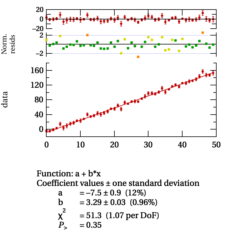
Some data scattered with gaussian noise about a line whose slope was set to \(3.23\) and whose offset was \(-5.7\).

Copy the code for jumble into the Procedure window (you can show the Procedure window either selecting it from the Window|Procedures menu or using Cmd/Ctrl-M). Click the Compile button at the bottom of the Procedure window and then enter Jumble(4, 1, 50) in the command line. Press return. If you have copied faithfully, and if you have successfully installed the HMC menu, you should see a figure similar to the one above.

Modifications

You can modify the slope and offset constants and try again, to see whether jumble behaves as expected. The slope and offset values are stored in the root data folder. You can either set new values from the command line like so:

slope = 4.32

or by bringing up the Data Browser (Cmd/Ctrl-B or from the Data menu), making sure that the checkbox next to Variables is checked, and then looking in the list of variables.

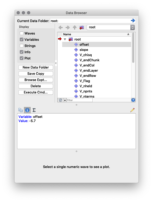
To edit a variable in the Data Browser, click the pencil icon.

Then issue the jumble command again to see if the new data are suitably modified.

Exploring parameter distributions

We have shown theoretically that when we weight each data point using its standard deviation in performing the least-squares fit, we expect the parameter values that result from the fit to be close to the true values, and that the uncertainty in the parameter values represent the standard deviation of their distribution. That is, if we were to gather statistics over many fitting trials, the values we deduce for the slope will be within one \(\sigma\) from the true value about 68% of the time.

To check this theory, we can run a large number nTrials of repetitions, and then make histograms of the normalized discrepancies between the parameter values d

// StudyParamDetermination(nTrials, mean_noise, std_noise, npts) runs a fit
// such as described in jumble many (nTrials) times, keeping track of how far
// from the true value of the fit parameter the determined value is. It
// then produces a histogram of the normalized values for both the slope
// and the offset fit parameter.
//
// Example: StudyParamDetermination(10000, 4, 1, 60)

Function StudyParamDetermination(nTrials, mean_noise, std_noise, npts)
  Variable nTrials, mean_noise, std_noise, npts

  // We will perform nTrials linear fits, each yielding
  // a slope and offset, which will differ from the true value
  // used to compute the noisy data by an amount we can record
  // as a multiple of the uncertainty in the fitted parameter
  // value. We record those errors in offset_error and slope_error.

  Make/N=(nTrials)/O offset_error, slope_error
  Make/D/N=2/O coeffs                 // slope and offset
  Make/O/N=(npts) data, amp, noise    // waves for the data and noise
  NVAR offset, slope                  // the global parameters

  Variable n
  for (n = 0; n < nTrials; n += 1)
    amp = mean_noise + gnoise(std_noise)  // the noise amplitude may vary
                                      // for each data point
    noise = gnoise(amp)               // draw the actual noise for each
                                      // point from a gaussian distribution
    data = offset + slope * x + noise

    // Perform the linear fit, putting the answers in the
    // wave coeffs. The /Q flag means to do it quietly, so
    // no delays from reporting to the history area and no dialogs.

    CurveFit/Q line kwCWave=coeffs data /W=amp /I=1

    WAVE W_sigma    // this wave is created automatically by CurveFit; it holds
                    // the uncertainties of the fit parameters

    // Record the normalized discrepancy in the fitting parameters

    offset_error[n] = (coeffs[0] - offset) / W_sigma[0]
    slope_error[n] = (coeffs[1] - slope) / W_sigma[1]
  endfor

  // Prepare a histogram for the slope errors and the offset errors

  Make/N=100/O slope_hist, offset_hist
  Histogram/B=1/C slope_error,slope_hist
  Histogram/B=1/C offset_error,offset_hist

  // Prepare graphs of the histograms
  Display/K=1 slope_hist
  HMC#FixGraph()
  ModifyGraph msize=2
  Display/K=1 offset_hist
  HMC#FixGraph()
  ModifyGraph msize=2

  // Lastly, shift the graphs so we see both of them
  GetWindow/Z kwTopWin wsizef
  MoveWindow V_right, V_top, 2*V_right - V_left, V_bottom
End

An example of the output of StudyParamDetermination is shown in the figure below.

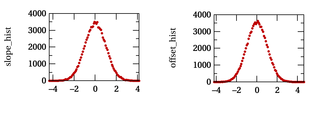
Histograms of the normalized discrepancy for the slope coefficient and the offset coefficient generated by StudyParamDetermination for 100,000 trials.

Exercises

1. Use StudyParamDetermination to generate histograms of normalized discrepancies. Then investigate the claim that the discrepancies are normally distributed. Do the distributions have the expected width? Hint: the uncertainty in a point of a histogram that has \(N\) counts should be \(\sqrt{N}\).
2. What does all of this mean? That is, summarize what all this simulation really signifies.

Example

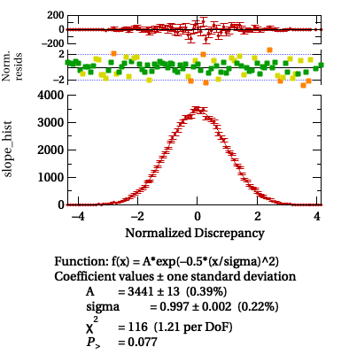
Do these data support the claim that the normalized discrepancies are normally distributed with the appropriate gaussian width?